2 Introducing R & RStudio
This chapter takes us from talking about data analysis to actually doing it. You will install and configure R and RStudio, the two main pieces of software we will use for the rest of the book.
Step by step, we will run our first commands in the console, write and save an R script, create a project folder, and bring a real dataset into R. You will learn how to see what objects are in memory, how to keep your workspace clean, and how to take a first look at a table of data with simple summary tools. When we finish, you will have a working setup and the basic moves needed for the exploratory work that begins in the next chapter.
The chapter covers
- Installing R and RStudio creates the computational environment needed for all subsequent statistical work.
- The RStudio interface organises code editing, console interaction, environment viewing, and file management into four main panes.
- RStudio Projects keep files organised and ensure code runs reliably across different computers and sessions.
- Core R concepts include functions, assignment with the arrow operator, object naming conventions, and the native pipe for connecting operations.
- Packages extend R’s capabilities, with
tidyverseandsgsurproviding the tools used throughout this book. - Essential global settings include blank-slate mode, native pipe shortcuts, and interface customizations that prevent common errors and improve workflow.
2.1 Installing R & RStudio
Before we download a single file, let’s untangle two names that often get lumped together: R and RStudio. They are related, but they are not the same, and knowing the difference will save early head-scratching.
RStudio is an integrated development environment (IDE); R is the statistical computing engine itself. R does every calculation, but we control and interact with R through RStudio.
Think of it like a car. R is the engine. RStudio is the driver’s seat, steering wheel, and dashboard. A car needs its engine to move, but most of the time the engine stays out of sight while we work the controls. The dashboard tells us what the engine is doing and lets us steer, accelerate, or brake.
You can run R without RStudio, but it can be clunky and difficult. Several alternative interfaces exist, yet RStudio is by far the most common and most liked. On the other hand, you cannot use RStudio without R; a dashboard without an engine goes nowhere.
So when we say install R, we almost always mean install R first and then install RStudio. Once both are installed, you will open RStudio, type commands, and let R do the heavy lifting behind the scenes. The rest of this book assumes exactly that workflow.
2.1.1 Installing R
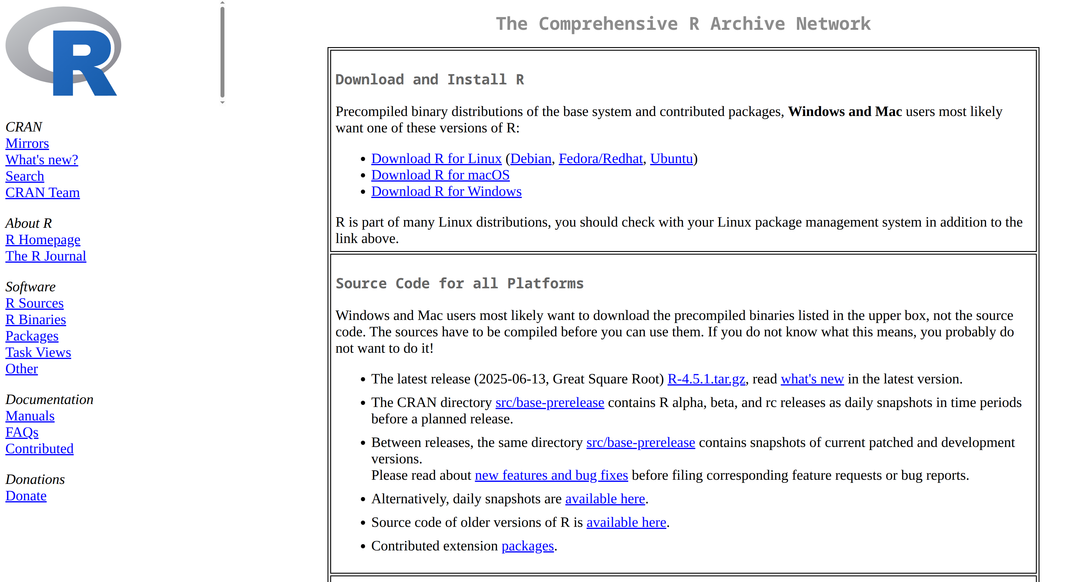
To install R, go to https://cran.r-project.org; see the screenshot in Figure 2.1.
At the top of that page, you will see Download and Install R. There are installers for three major platforms: Windows, macOS, and Linux. We will assume you are using either Windows or macOS (and may not even have heard of Linux), so we will walk through the instructions for those two platforms.
2.1.1.1 Windows
- Click Download R for Windows.
- Choose the base or install R for the first time link. Both lead to the same page; ignore the other options for now.
- Click Download R-4.x.y for Windows, where x.y is the current version. For example, as of 5 January 2026 the current version was R-4.5.2. Save the file.
- Double-click the downloaded
.exeinstaller. If Windows SmartScreen asks whether to run the file, choose Run anyway. - Accept the default language (English or your system language) and licence. R is distributed under the GPL, so it is free to use.
- When asked about 32-bit vs. 64-bit, leave the default 64-bit ticked. Only very old machines need 32-bit.
- Accept the default install path (
C:\Program Files\R\R-4.x.y\). Click Next on all component screens; the defaults are sensible. - Finish the wizard. A new Start-menu group called R appears. Launch this to verify the installation. This minimal interface is unnecessary once RStudio is installed, but opening it confirms that R works. Close it before installing RStudio to avoid conflicts.
2.1.1.2 macOS
- Click Download R for macOS.
- Download the installer for the latest version. You will see two installers: one for Apple Silicon and one for Intel. Most modern Macs use Apple Silicon; older models use Intel. Each installer ends in
.pkg. - Double-click the
.pkgto launch Apple’s installer. You may need to enter your macOS password. - Accept the default destination disk and click Install.
- Gatekeeper might flag the package as “unidentified developer”. Choose Open Anyway.
- When the installer finishes, R lives in
/Library/Frameworks/R.framework. You never need to touch that folder directly. - Open your Applications folder and double-click the R icon to verify the installation. Close it before installing RStudio.
2.1.2 Installing RStudio Desktop
As mentioned above, RStudio is an Integrated Development Environment (IDE) for R. Bare-bones R works, but RStudio’s multi-pane window, auto-completion, file browser, and other features make life much easier.
Here are the step-by-step instructions for installing RStudio Desktop on Windows and macOS.
2.1.2.1 Windows
- Go to https://posit.co/download/rstudio-desktop.
- Click Download RStudio Desktop for Windows (a
.exe, e.g.,RStudio-202X.XX.X-XXXX.exe). - Locate the installer in your Downloads folder and double-click it.
- If User Account Control asks for permission, click Yes.
- In the Welcome to RStudio Setup wizard, click Next.
- Accept the default installation location (
C:\Program Files\RStudio) and click Next. - Accept the default Start-menu folder name and click Install.
- When installation completes, click Finish.
- Open the Start menu, search for “RStudio”, and launch the application.
2.1.2.2 macOS
- Go to https://posit.co/download/rstudio-desktop.
- Click Download RStudio Desktop for macOS (a
.dmg, e.g.,RStudio-202X.XX.X-XXXX.dmg). - Locate the
.dmgin your Downloads folder and double-click it. - Drag the RStudio icon into the Applications folder alias.
- Close the installer window and eject the RStudio disk image. You may delete the
.dmgif you wish. - Open the Applications folder and double-click the RStudio icon. The first launch may prompt for confirmation; click Open.
2.2 Guided tour of RStudio
Opening RStudio for the first time can be overwhelming. It may look a bit like the instrument panel in a plane’s cockpit; what everything does is not at all obvious. Once you start using RStudio regularly, it soon becomes second nature, but at the beginning a guided tour helps.
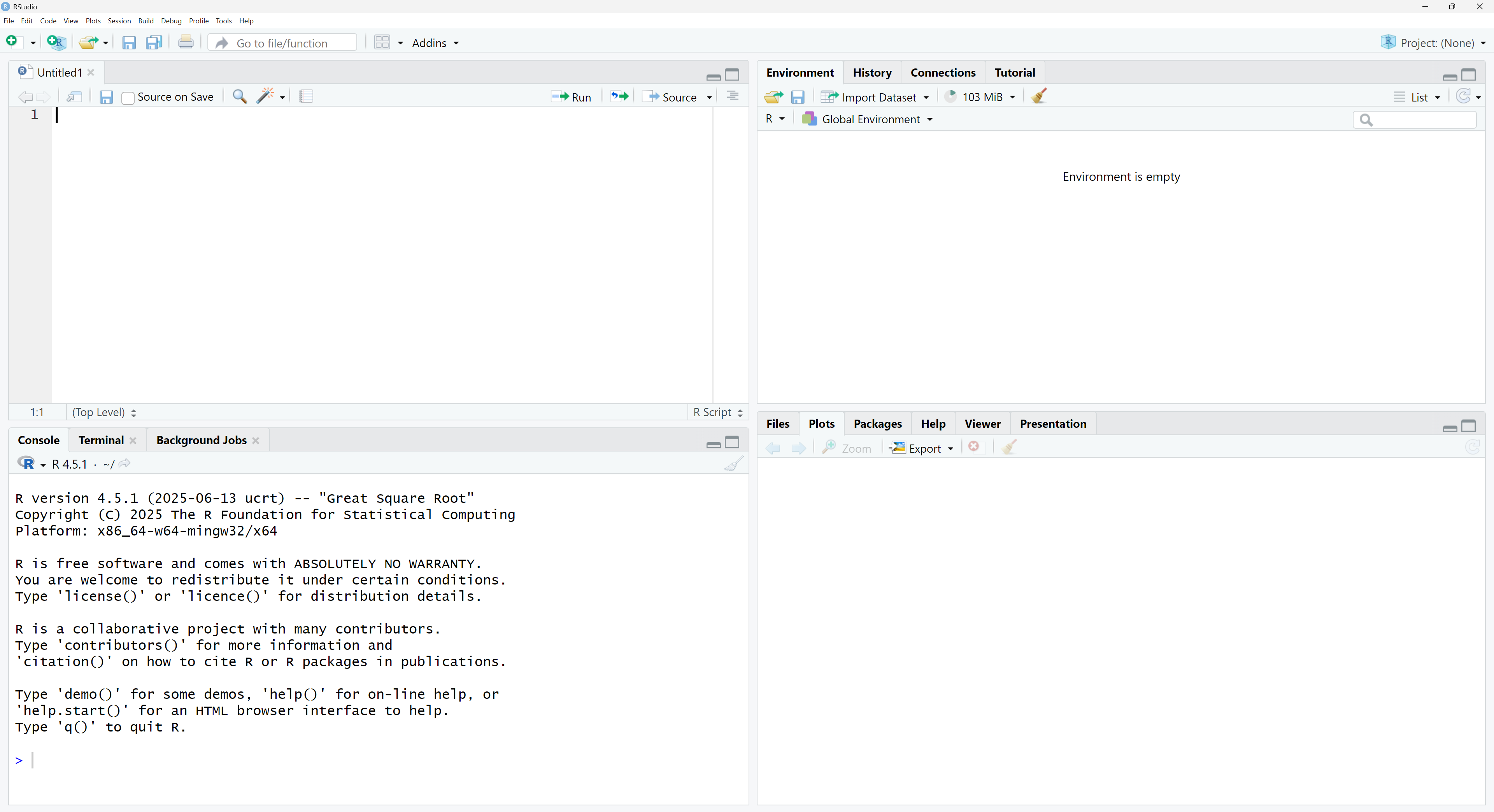
Most users work in the four-pane layout shown in Figure 2.2. Because that layout is the norm, the tour below assumes four panes.
The four panes are:
- Bottom-Left: Console
- Top-Left: Editor
- Top-Right: Environment / History
- Bottom-Right: Files / Plots / Packages / Help / Viewer
You can rearrange them under Tools > Global Options > Pane Layout, but the default works well.
- Console Pane (Bottom-Left)
-
This pane has three tabs — Console, Terminal, and Background Jobs — but the Console is the one you will use every day. It is the direct interface to R: type a command after the
>prompt and press Enter to run it immediately. Printed results, warnings, and error messages appear here. The Terminal tab opens a system shell (Command Prompt on Windows, a Unix shell on macOS); useful for advanced tasks but not needed in ordinary work. Background Jobs manages long-running tasks, another feature for experienced users. - Editor Pane (Top-Left)
-
Your main workspace for writing and saving code. R scripts (
.R) are the most common file type, but you can also edit R Markdown (.Rmd), Quarto (.qmd), and other plain-text documents. Scripts make your analysis reproducible because every command is stored in a file you can rerun later. The editor supports syntax highlighting, code completion, and smart indentation. Multiple files open as tabs, and you can send selected lines — or the whole script — to the console with Ctrl + Enter (Windows) or Cmd + Enter (macOS). - Environment / History Pane (Top-Right)
- Helps you track what is in your current R session. The Environment tab lists every object you have created or loaded: data frames, vectors, functions, and so on. Click an object (especially a data frame) to view it in the editor. The broom icon clears the environment, handy for starting fresh, and import buttons let you load data from CSV, Excel, SPSS, SAS, or Stata files. The History tab records every command you have run; you can resend commands to the console or editor with a click. Other tabs — Connections, Build, Git, and others — support database work, package development, or version control, but most beginners can ignore them.
- Files / Plots / Packages / Help / Viewer Pane (Bottom-Right)
-
A collection of tools for project management, visualisation, package handling, and documentation. Files is a mini file-browser for your project directory. Plots shows graphs you create, lets you step through earlier plots, clear the history, or export the current plot to PNG or PDF. Packages lists installed libraries and provides buttons to install new ones from CRAN or update existing ones. Help displays documentation for functions, datasets, and packages; typing
?function_namein the console opens the relevant help page here. Viewer renders local web content; most users rarely need it, so we will skip it for now.
2.3 Installing packages
R ships with a robust toolkit for statistics, data manipulation, and plotting. For many tasks that might be all you ever need. What makes R extraordinary — and one reason it is so widely used — is the thousands of add-on packages contributed by users and researchers. CRAN, the main public repository, now hosts well over 20,000 such extensions (exactly 22,953 as of 5 January, 2026), covering almost every modern method in statistics and data analysis.
To install any R package, open the Packages tab in the lower-right pane and click Install. The dialogue in Figure 2.3 appears.
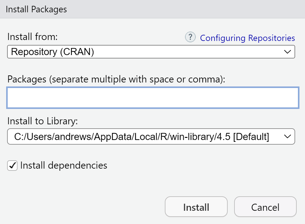
Type a package name in the box and press Install. You can also enter several names, separated by spaces or commas. When you do this, in the console, RStudio runs
install.packages("package_name")so anything you do in the dialogue could equally well be typed into the console.
Whenever you install a package, R automatically installs its dependencies, which are any other packages it needs to work. The process is recursive, so one command can pull in dozens of additional libraries.
2.3.1 Installing the packages for this book
This text relies most heavily on two packages:
tidyverse: a meta-package that installs the data-wrangling and plotting workhorses (dplyr,ggplot2,readr, and friends).sgsur: the companion package for this book. It supplies example datasets, helper functions, and small utilities used in later chapters.
To install all the packages needed in this book, do the following. In the Install dialogue box, type sgsur and click Install, or else run in the console
install.packages("sgsur")After the sgsur installation finishes, in the console, run
sgsur::install_extras()Press Enter and watch the scrolling log as R downloads all required packages and their dependencies.
When everything is finished, click the circular Refresh icon at the top of the Packages tab. Your library list is now longer; use the search box to filter by name, tick a check-box to attach a package, or untick to detach it.
In general, whenever you need a new package, you can either
- click Install in the Packages tab, or
- type
install.packages("newpackage")in the console.
Both routes do exactly the same job so choose whichever feels quicker.
2.3.2 Loading packages
After a package has been installed, it sits passively on your disk. R will not use it until you load it for use in your current R session. The standard way to do that is to call library(). For example, to load up the tidyverse and sgsur packages, which we will rely on heavily throughout this book, we do the following:
library(tidyverse)
library(sgsur)
Sometimes when packages load, they do so quietly. Other times they produce messages. The sgsur package will load silently, but calling library(tidyverse) produces the following chatty output:
── Attaching packages ───────────────────────────────────── tidyverse 2.0.0 ──
✔ ggplot2 3.4.0     ✔ purrr   1.0.2
✔ tibble  3.2.1     ✔ dplyr   1.1.3
✔ tidyr   1.3.0     ✔ stringr 1.5.0
✔ readr   2.1.4     ✔ forcats 1.0.0

── Conflicts ─────────────────────────────────────── tidyverse_conflicts() ──
✖ dplyr::filter() masks stats::filter()
✖ dplyr::lag()    masks stats::lag()
ℹ Use the conflicted package to force conflicts to become errors
The first line — Attaching core tidyverse packages — tells you that the meta-package has just attached eight individual libraries (ggplot2, dplyr, readr, and so on). Each green tick reports success. The second block headed Conflicts may look ominous at first glance. However, nothing has gone wrong. It is simply a courtesy notice that a few function names exist in more than one package and it tells you which function takes precedence. In this case, it tells you that functions named filter and lag exist in both the dplyr and the stats packages, and now dplyr takes precedence. For example, when you call filter(), by default it will call dplyr’s filter(). If on a rare occasion you actually need the stats version of filter or lag, you can call the function using the stats package name followed by a double colon: stats::filter() or stats::lag(). This bypasses the default order and calls the function directly. In fact, it is always possible to use any function in any package this way, even if it is not loaded up with library(). However, this is rarely done. Throughout this book, we will nearly always use library() to load a package’s functions.
If a package prints a message banner, it appears only the first time you load a package in a session. A second call to library(tidyverse) does nothing because R sees that tidyverse is already loaded and so it does not reload it.
At any moment, you can easily see what packages are installed or loaded in the Packages tab in the lower right pane in RStudio. Make sure to press the refresh icon in the upper right of the tab to ensure you have the up-to-date list. The list of packages you see, which you can search through using the search bar, will tell you what is installed. On the left of each item in the list is a tick box. If this is ticked, then the package is loaded. If you manually tick an unticked box, R then runs library() for that package. While that might seem handy, we recommend always typing your library() calls explicitly in your R scripts in order to have a complete record of all the code needed in any analysis; a point we elaborate below.
Note 2.1: Could not find function
From time to time, you will undoubtedly encounter an error message like this:
Error in foobar() : could not find function "foobar"What this is telling you is that you are calling a function that does not exist. There are most likely three reasons for this:
- You mistyped the name of the function. For example, instead of typing
sqrt(42), you typedSqrt(42), or made some spelling mistake, and so on. - You typed the function correctly, but have not yet loaded the package. For example, you called
glimpse(), which is part ofdplyr, but have not yet donelibrary(tidyverse). - You are trying to use a function from a package that is not yet installed. In that case, first install the package as described above and then load it with
library().
2.4 Changing global settings
Before you write even a single line of code, spend a few minutes in Tools︎ > Global Options.
Changing a handful of defaults now prevents several common headaches later or otherwise makes your life easier. Everything below is safe for beginners and pays off immediately.
2.4.1 Set the blank-slate rule
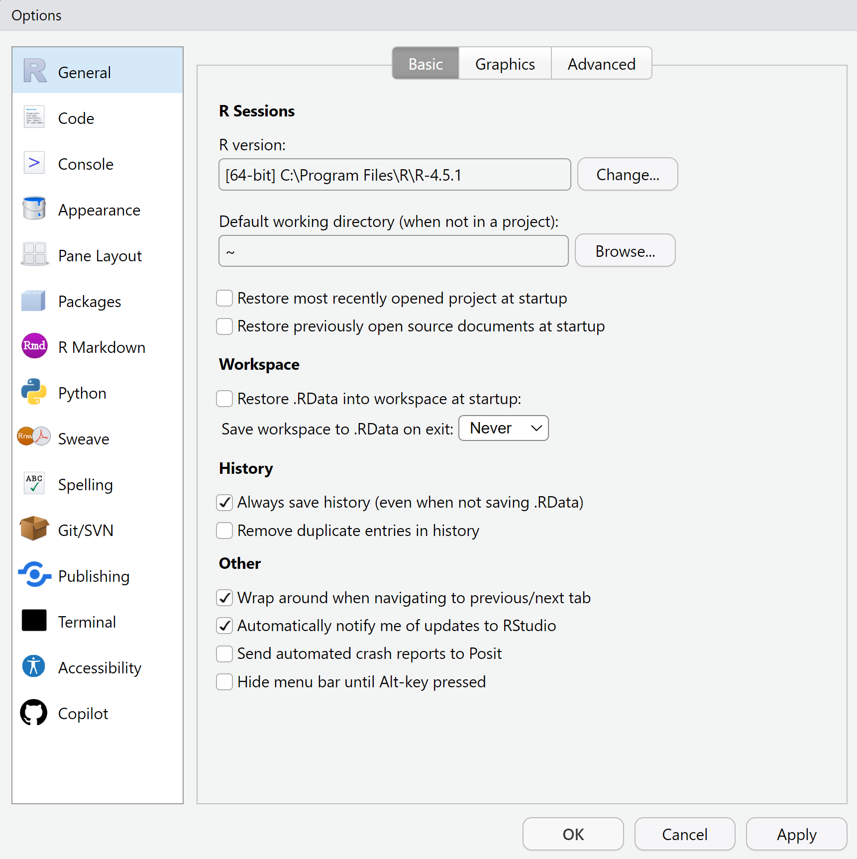
R comes with a convenience feature that remembers every object in your workspace when you quit and silently restores them next time. It sounds handy, but experienced users recommend turning it off. Old objects linger, mixing yesterday’s experiments with today’s work so you can’t tell which results are current and which are relics. Worse, your script is no longer a complete recipe: if it depends on an object resurrected from an earlier session, the code appears to work on your machine but fails for anyone else, even for your future self a month later on a new laptop.
The fix is to set the blank-slate rule: start every session with an empty workspace and let the script rebuild everything. Open Global Options > General, clear Restore .RData into workspace at start-up, and set Save workspace to .RData on exit to Never. With those two changes the script becomes the single source of truth; if a command is not in the file, it doesn’t happen.
2.4.2 Use the native pipe
Later in this chapter we will introduce pipes, a feature that lets you write a multi-step data transformation as a clear, left-to-right sentence. Pipes appear throughout this book, so a little setup now pays off quickly.
Since R 4.1 the base pipe operator |> is built into R itself. An older pipe, %>%, comes from the magrittr package and is widely used in the tidyverse. For almost every task the two behave the same, but %>% works only after you load the right packages, whereas |> is always available. For that reason we — and many other users — recommend making |> your default pipe.
Set a handy shortcut by opening Code > Editing and ticking Use native pipe operator. After that, Ctrl/Cmd + Shift + M inserts |> with the correct spacing, making a pipe as easy to type as a plus sign.
2.4.3 Add visual cues while you type
Small colour hints help you spot errors before you run the code.
- Code > Display > Rainbow parentheses colours each level of nesting, so a missing bracket jumps out immediately.
- In the same panel, turn on Rainbow indent guides and Show line numbers. Line numbers make it easier to discuss code in class, and indent guides stop you getting lost inside long functions.
- Still in Display, tick Soft-wrap R source files if you use a narrow laptop screen; it prevents horizontal scrolling.
2.4.4 Theme, font, and zoom
Staring at code for hours is easier when the colours suit your eyes. Open Appearance and try out different Editor Themes. Try a dark theme such as Cobalt (our personal favourite) or stick with the default light TextMate. There is no right answer; just experiment and see what you prefer. While you are in Appearance, play with the editor font size, and/or change the zoom size, until the scale feels comfortable. Also remember View > Zoom In (Ctrl/Cmd + =) / Zoom Out (Ctrl/Cmd + -) can be used to change the zoom on the fly.
That is all the configuration most beginners need. Everything else — panel layout, custom keybindings, Git integration — can wait until you have a genuine reason to change it.
2.5 Using RStudio projects
Whenever you work in RStudio, we strongly recommend using an RStudio Project. An RStudio Project is simply a folder that holds all the files — data, scripts, and results — for a specific analysis, plus a small .Rproj file that tells RStudio, “this folder is a project.” When you open or switch to a Project, RStudio automatically sets R’s working directory to that project folder, making it the default location for reading and writing files. It also loads a hidden history file that records every command you have run in that project, so your past work appears in the History tab.
Projects are a straightforward idea but extremely useful for beginners and experienced users alike. Because every analysis lives in its own folder, your work stays organised and easy to find. More importantly, the project’s working directory keeps your code reproducible and portable: any file path you write can be relative to the project root, so your script still runs when you move it to another computer. If this benefit is not obvious yet, it will become clear once we start writing code that reads or writes files. A project also remembers where you left off — open files, command history, even pane layout — so you can resume work instantly.
To create a new project:
- Choose File > New Project.
- Select Existing Directory if you already have a folder, or New Directory > New Project to create a fresh one.
- Give the folder a short, descriptive name: for example,
sgsur_textbook. - Leave Open in new session ticked and click Create Project.
RStudio opens a new window; the title bar and the top-right corner both show the project name. Inside the Project folder you will see sgsur_textbook.Rproj. Opening that file later restores the project exactly as you left it. You can also switch projects with File > Open Project or pick from File > Recent Projects.
For the remainder of this book we will assume you are working in an RStudio Project named sgsur_textbook.
2.6 First steps using R
Now that you have explored RStudio’s layout, adjusted key options, and created a project to keep your work organised, you are ready to take your first steps in R itself.
The Console pane, bottom-left in the default layout, is your direct interface to R. Type code after the > prompt, press Enter, and R executes it immediately, printing the result on the next line.
Begin with the console as a simple calculator. Click in the Console pane, type
2 + 2and press Enter. R prints
[1] 4The tag [1] indicates that this is the first (and here only) element of the output; the value itself is 4.
Spacing is flexible. The expressions 2+2, 2 +2, 2+ 2, or even 2 + 2 all yield the same result. Spaces exist purely to make code easier for humans to read; R ignores them.
To get the hang of typing commands and seeing results, try the following calculations. For each line, type the code exactly as shown and press Enter.
# 5 minus 10
5 - 10
[1] -5# 2 times 3
2 * 3[1] 6# 4 divided by 6
4 / 6[1] 0.6666667# 10 to the power of 2
10 ^ 2[1] 100Calculations like these in R work much like those on a hand-held calculator. See Note 2.2 for an overview.
Note 2.2: Arithmetic in R
Arithmetic in R works much like an ordinary calculator:
+addition-subtraction*multiplication/division^(or**) exponents
Round brackets () group terms, and R follows the standard order of operations (BODMAS or PEMDAS): brackets first, then exponents, then multiplication and division, then addition and subtraction.
For example:
(10 + 4) * (2 ^ 3) / (8 - 1)[1] 162.6.1 Functions
Calculations with +, *, and other operators are useful, but most of R’s power comes from functions. Think of a function as a command: you supply input, it does its job, and it returns a result. Run a function by writing its name followed by parentheses, placing the input inside the parentheses.
log(10) # natural logarithm of 10[1] 2.302585sqrt(25) # square root of 25[1] 5abs(-3.4) # absolute value of -3.4[1] 3.4Each line sends a number into the command, and R returns an answer.
Some functions take multiple inputs and return a single value:
log(10, 2) # logarithm of 10 to base 2[1] 3.321928Here 10 is the number and 2 is the base.
Other functions accept one input value and return several values:
rnorm(3) # three random draws from a normal distribution[1] -2.6732893 -0.1664729 -0.1597477The input 3 tells rnorm how many random numbers to generate; the output is a set of three numbers.
R has a vast number of functions; probably hundreds of thousands when you include add-on packages. Throughout this book we will see many of them in action. Each one does something different, but all follow the same principle: data in → data out.
Tip 2.1: What does a command do? Use
?command.
Whenever you wonder what a function does, type a question mark before its name — for example, ?log — and RStudio opens a help page that explains the input it expects and the output it returns.
2.6.2 Assignment
In every example so far, the result appeared on the screen and then vanished from memory. Usually, you will want to store results for later use. You do this with assignment: the assignment operator <- (< followed by -) puts whatever is on the right into the name on the left.
x <- 2 + 2 # store the result of 2 + 2 in xBecause x now holds a value, you can treat it as if it were that value:
x # prints 4[1] 4and use it in further calculations:
y <- x * 3
y            # prints 12
[1] 12To the right of <- can be any R expression such as a function call, calculation, data structure, or simple number:
my_number  <- 10          # my_number gets 10
sum_result <- 5 + 3       # sum_result gets 8
log_result <- log(100)    # log_result gets log of 100
The general pattern is
result_name <- expressionread as result_name is assigned the value of expression.
While result_name = expression often works, <- is the idiomatic assignment operator in R and avoids confusion with situations where = is required.
Tip 2.2: What’s in a name?
Names for stored results can include uppercase and lowercase letters, digits, periods (.), and underscores (_), but must follow a few rules:
- Start with a letter or a period; if a period is first, the next character cannot be a digit.
- Exclude other symbols such as
-,!, or@. - Names are case-sensitive:
myresult,myResult, andMyResultare all different. - Avoid reserved words like
if,else,for,while, orfunction(?Reservedshows the full list). - Do not reuse common function names such as
sum,mean, orsd.
Best practices for variable naming:
- Descriptive: Use names that clearly indicate content:
total_salestells you more thants1. - Snake case: (e.g.,
student_height) is most common in R and what we use in this book. - Camel case: (e.g.,
studentHeight) works fine but is less common in R. - Avoid periods: (e.g.,
student.height) periods can clash with R features; prefer underscores.
Think of naming as writing notes to your future self and collaborators. Clear, consistent names make your code easier to read, debug, and share.
2.6.3 More than numbers
So far every object you have created has been a single number, but R can store many other kinds of information. An object might hold text ("Hello"), a logical value (TRUE or FALSE), a collection of values of the same type (known as a vector), or many other specialised structures.
For everyday data analysis, the workhorse object is the data frame: a rectangular table where each column is a vector (numbers, text, or dates) and each row is an observation. Almost everything in this book revolves around creating, inspecting, and transforming data frames, so we will turn to them soon.
For now, keep in mind that when you assign a result with <-, the “result” can be any of these object types, not just single numbers.
2.6.4 The pipe
The pipe operator |> is a small piece of R code that lets you pass a result from one function straight into another function. Once you get used to it, you will probably find it makes reading and writing code, especially code that involves several steps in succession, much easier to read and understand.
To understand it, start with a single number.
x <- 42Calling a function, such as calculating the logarithm, the usual way looks like this:
log(x)[1] 3.73767The pipe version puts the value first and the function after:
x |> log()[1] 3.73767Both lines return exactly the same answer. You can read the pipe aloud as “and then”. In more detail, you can read it as “the thing on the left of |> is sent to the function on the right”.
Pipes become helpful when more than one transformation is needed. Suppose we want the logarithm of the square root of the absolute value of the logarithm of x. The normal way of doing this is to use nested functions like this:
log(sqrt(abs(log(x))))[1] 0.6592312By contrast, the pipe form is like this:
x |> log() |> abs() |> sqrt() |> log()[1] 0.6592312Read the pipeline from left to right: take x and then calculate its logarithm, then the absolute value, then the square root, and then the logarithm again.
The two lines give the same numeric result, but the piped version contains no nested function, is arguably easier to read, and is easier to extend or edit. We will return to pipes in the data-wrangling chapter where they let us chain several tidyverse verbs into clear, readable pipelines.
Tip 2.3: This is not a pipe
In R code, you will often come across %>%, which is known as the tidyverse or magrittr pipe. It is loaded automatically when you load tidyverse and many other packages. For most practical purposes, %>% behaves just like |>. Like others, we will use |> by default just because this now is part of the R language and so requires no extra packages to be loaded.
2.7 R scripts
A single line in the console is perfect for a quick calculation or for testing an idea, but serious work soon demands something more permanent. An R script is that something: a plain-text file that records every command you want to keep. Storing your analysis in a script has three advantages. First, you can rerun the whole sequence tomorrow — or next year — without re-typing. Second, you can share the file so a colleague (or future you) can reproduce every step. Third, a script is easy to revise: you can read, edit, and improve it whenever your data or ideas change.
2.7.1 Creating and saving an .R script
Choose File > New File > R Script. A new tab opens in the Editor pane. Think of this editor exactly as you would a blank document in Word or an empty email: you type plain text, press Enter to start a new line, and nothing happens in R until you tell it to run the code.
Type the following in the blank script:
x <- rnorm(50)
mean(x)
sd(x)
Press Ctrl/Cmd + S (or File > Save) and name the file sim_summary.R.
Assuming you followed our earlier advice and are working inside the sgsur_textbook project, the save dialogue automatically points to that project folder, and so when you save it there, this script lives alongside your data and results.
2.7.2 Running code from a script
Running code in the editor is as easy as in the console, but you have several options.
Ctrl/Cmd + Enter: Place the cursor anywhere on a line, and press Ctrl/Cmd + Enter. RStudio copies that line to the console, runs it, and moves the cursor to the next line. Optionally, you can highlight several lines at once, and Ctrl/Cmd + Enter runs the whole block.
Run button: the green Run button at the top of the editor does the same thing as Ctrl/Cmd + Enter for whatever line the cursor is on or for a highlighted block of lines. Click the small arrow beside it to choose Run Section or Run Selected Lines.
Source – click Source (or press Ctrl/Cmd + Shift + Enter) to send the entire file to R in one batch. The console shows every command and its output, making this the fastest way to confirm that the whole script runs correctly from scratch.
A typical workflow is to experiment line-by-line with Ctrl/Cmd + Enter while writing, then use Source to check that the complete script still works after bigger edits.
2.7.3 Code comments
Comments are notes to yourself or anyone else who reads your code. In R, comments start with a # (hash symbol). Anything you write after a # on a line is completely ignored by R when it runs your code. It’s just plain text for humans.
Here’s an example:
# generate 50 random values from a normal distribution
# with mean of 0 and standard deviation of 1
x <- rnorm(50)

# basic summary statistics
mean(x)      # average
sd(x)        # standard deviation
Comments are extremely helpful in all coding. When you come back to your code next week, next month, or next year, you might forget why you made certain choices. Comments serve as reminders. Instead of just saying what a line of code does (which the code itself often shows), use comments to explain why you wrote it that way, what problem it’s solving, or what assumptions you’re making. This is crucial for understanding. You can temporarily “comment out” lines of code (add a # in front) to prevent them from running, which is a common trick for finding errors. If someone else needs to understand or use your code, comments are invaluable for guiding them through your thought process.
For beginners, the advice is to comment a lot. Don’t worry about commenting too much; it’s better to over-explain early on. As you gain experience, your commenting style will naturally become more concise.
2.7.4 Sections
You can divide your code into sections by inserting a # at the start of the line, followed by a title or label, followed by a series of dashes to the end of the line as in the following examples:
# simulate data ----------------------------------------------------------------------------

# generate 50 random values from a normal distribution
# with mean of 0 and standard deviation of 1
x <- rnorm(50)

# descriptive statistics -------------------------------------------------------------------

# basic summary statistics
mean(x)      # average
sd(x)        # standard deviation
You can insert a section quickly with Ctrl/Cmd + Shift + R or Code > Insert Section, which will bring up a dialogue box where you enter the section’s title or label.
In RStudio, a small arrow to the left of the section can be used to collapse (hide) or expand (unhide) all the code in that section. It also provides a navigation menu to jump between sections in the Document Outline (upper right of the editor). You can run all the code in a section by choosing Code > Run Region > Run Code Section.
2.7.5 Line breaks
When writing R code, you’ll often encounter situations where a single line becomes too long to read comfortably. R allows you to break long lines across multiple lines to improve readability.
R automatically continues to the next line when it detects that a statement is incomplete. This happens naturally when you have, for example, unclosed brackets:
mean(     # opening bracket
  x
)         # closing bracket; end of statement
[1] 42Likewise, it will occur when you have operators, like +, -, at the end of the line:
total <- 1 + 2 +
         3 + 4 +
         5
It also occurs with pipes:
log(42) |>
  sqrt() |>
  log()
[1] 0.6592312Breaking lines strategically makes your code much easier to read and debug, especially when working with complex functions or data pipelines. We will see many examples throughout this book.
2.7.6 Tidying code
Consistent spacing and indentation make scripts easier to read. Select some code and choose Code > Reformat Selection or press Ctrl/Cmd + Shift + A and RStudio will reformat this code to make it more readable. RStudio’s built-in formatter relies on the styler package. If you followed our advice earlier and installed all packages required or used in this book with sgsur::install_extras, then you will have it installed already. If it is not installed you may be prompted to add it the first time you use this feature.
2.7.7 Script versus console
Think of the console as your scratch pad: a place to experiment, try a function, or inspect an object. Nothing there is permanent unless you copy it elsewhere, so mistakes cost nothing.
The script is your definitive record. As soon as a console line proves useful, paste it into the script, add a brief comment, and save. Over time, the script becomes a clear narrative from raw data to final results, while the console remains littered with tests and false starts.
A practical rhythm emerges:
- Prototype a line in the console.
- Move it into the script when it works.
- Press Source now and then to ensure the entire script still runs cleanly.
Follow that rhythm and, by the time you finish an analysis, you will have a tidy, reproducible script you can trust, share, and revise whenever new data arrive.
2.8 Importing data into R
The first step in any data analysis is importing our data. Data files come in a bewildering variety of formats — comma-separated text (.csv), tab-delimited text (.tsv), Excel workbooks (.xlsx), SPSS system files (.sav), Stata files (.dta), SAS transport files (.xpt), and many more — but you can relax: with the right helper packages, R can read them all. In this book, for convenience, we mostly use built-in datasets that ship with our sgsur package, but the mechanics of reading data from an external file into an R session are so fundamental that we should rehearse them before moving on.
If you have not already done so, use library() to load the tidyverse and sgsur packages:
library(tidyverse)
library(sgsur)
The tidyverse gives us the read_csv() function from the readr package, which is a very widely used function in R. The sgsur package ships with some demonstration data files and a function to copy these files into your working directory.
Assuming you are working inside an RStudio project — as strongly recommended earlier, see Section 2.5 — your working directory is set to the project folder and so the following command will copy the screensurvey.csv file shipped with sgsur into your project folder:
copy_extdata("screensurvey.csv") # writes the file to your project rootYou can verify that this worked by going to the Files tab in the lower right pane in RStudio, pressing the refresh icon, and you should see screensurvey.csv listed.
With the file in place, we can read it into R:
screen_df <- read_csv("screensurvey.csv")You will notice that the console prints a short progress report: how many rows were read and which column types were guessed. These lines are normal; they are not warnings, just friendly feedback that the parser succeeded.
Typing the screen_df name shows a rectangular data structure:
screen_df# A tibble: 60 × 5
id age gender scr_hrs happy10
<dbl> <dbl> <chr> <dbl> <dbl>
1 1 54 F 7 4
2 2 18 F 6.2 6
3 3 42 F 2.2 7
4 4 27 F 3.8 6
5 5 53 M 5.9 6
6 6 35 F 2.3 8
7 7 64 F 2.9 8
8 8 41 M 5.7 4
9 9 24 M 6.4 5
10 10 53 M 5.4 7
# ℹ 50 more rowsThe header line tells you that the object is a tibble or data frame (see Note 2.3), with 60 rows and 5 variables.
Note 2.3: Data frames and tibbles
A data frame is the most common way to work with data in R. It is a rectangular data structure just like a spreadsheet; it has rows and columns, where each row represents an observation (like a person or measurement) and each column represents a variable (like age, height, or name).
A tibble is basically a modern, improved version of a data frame. It’s part of the tidyverse and does almost everything a data frame does, but with some nice enhancements that make it easier to work with. In particular, tibbles show you a neat preview of your data (first 10 rows, column types, etc.), and have some other nice features that make it easier to look at your data. For this reason, throughout this book, we will always use tibbles.
In almost every respect, however, you can treat a tibble as just a regular R data frame, and in fact we will use the terms interchangeably in this book.
Listing every data import function in R and its package ecosystem would take pages, yet the principles are very similar to the example just seen. For example, we can use a function read_excel to read Excel workbooks; read_sav to read SPSS data files; read_dta to read Stata files, and so on. Once the data is read in, you manipulate it in exactly the same way.
That is all we need at this stage: files live on disk, library(tidyverse) gives us the read_csv import function; the call to read_csv("screensurvey.csv") reads in the data from the file, and the result is a tibble ready for exploration. The next chapter begins that exploration in earnest.
2.9 Further reading
Richard Cotton’s Learning R: A Step-by-Step Function Guide to Data Analysis (Cotton, 2013) provides a gentle, beginner-friendly introduction to R fundamentals, covering installation, basic operations, and core programming concepts.
Garrett Grolemund’s Hands-On Programming with R (Grolemund, 2014) takes readers from the console through scripts, functions, and projects with extensive practical examples.
2.10 Chapter summary
Rand RStudio are distinct but complementary:Ris the statistical computing engine, while RStudio provides the interface, editor, and project management tools that makeRaccessible and productive.- RStudio’s four-pane layout organises console interaction, code editing, environment viewing, and file management, with menus providing access to installation, configuration, documentation, and workflow commands.
- Critical global settings include blank-slate mode to ensure scripts are the single source of truth, native pipe shortcuts for streamlined workflows, and visual aids like rainbow parentheses to catch errors early.
- RStudio Projects organise analyses into self-contained folders with automatic working directory management, making code portable, reproducible, and easy to resume after interruptions.
R’s core operations include functions that transform inputs to outputs, assignment with the arrow operator<-to store results, and the pipe operator|>for chaining multi-step transformations into readable left-to-right sequences.- Packages extend
R’s capabilities infinitely, withtidyverseproviding data wrangling and visualisation tools andsgsursupplying datasets and utilities for this book, both loaded withlibrary()after installation. Rscripts are plain-text files that record every command, enabling reproducible workflows where the entire analysis from raw data to final results can be rerun, shared, and revised at any time.- Importing data from CSV, Excel, SPSS, Stata, and other formats into tibbles (modern data frames) is straightforward with
tidyversefunctions, creating rectangular structures ready for analysis.