library(tidyverse)
library(sgsur)8 Multiple linear regression
In Chapter 7, we focused on simple linear regression, which examines the relationship between one predictor variable and an outcome variable. This chapter extends that framework by using several predictors at once. This is called multiple linear regression.
Multiple linear regression builds naturally on simple linear regression. Most or all of the theoretical concepts we covered earlier still apply. Likewise, the code and general workflow in R remain very similar or even unchanged. However, multiple linear regression is not the same as running several simple linear regressions at once. It allows us to address important questions that are not possible with simple linear regression alone.
Multiple linear regression lets us study the combined explanatory power of sets of predictors. Simple linear regression shows us how much the outcome changes as one predictor changes, but multiple linear regression shows us how the outcome changes as combinations of predictors change. Similarly, while simple linear regression allows us to predict the outcome from one predictor, multiple linear regression allows us to predict the outcome from a combination of predictor values. Separate simple regressions cannot answer such joint questions because they examine each predictor in isolation and ignore the way the predictors work together.
Multiple linear regression also allows us to see how the outcome changes with one predictor after controlling for the effect of other predictors. With a simple linear regression, we measure the overall association between the one predictor and the outcome, but that includes the effect of other variables that are correlated with the predictor. For example, if richer countries tend to have better healthcare, and better healthcare leads to more happiness overall, a simple regression with happiness as the outcome and income as the predictor attributes some of the influence of healthcare to income. On the other hand, a multiple regression using both income and healthcare as predictors separates these influences by estimating the effect of each predictor after accounting for the other. The income coefficient in that model therefore reflects only the part of income that cannot be predicted from healthcare. This adjustment is necessary if we want an unbiased estimate of how income itself relates to happiness rather than a mixture created by correlated variables.
The chapter covers
- Multiple linear regression extends simple regression by modelling outcomes as functions of several predictors simultaneously rather than in isolation.
- Each coefficient estimates a predictor’s partial effect while holding other predictors constant, separating unique from shared contributions.
- Model fit statistics like \(R^2\), adjusted \(R^2\), and F-tests quantify how much variation predictors collectively explain.
- Standardized coefficients enable direct comparison of effect sizes across predictors measured on different scales.
- Multicollinearity occurs when predictors are highly correlated, inflating standard errors and destabilising coefficient estimates, diagnosed using variance inflation factors.
- Model comparison using F-tests and information criteria determines whether adding predictors meaningfully improves explanatory power.
8.1 Beyond income: Multiple predictors of happiness
In Chapter 7, we used the whr2025 dataset, which included countries’ average life satisfaction and their per capita GDP (a measure of the country’s wealth). This data came from the 2025 edition of the World Happiness Report. In this chapter, we will use a related dataset, whr2024:
whr2024# A tibble: 131 × 9
country happiness gdp lgdp support hle freedom generosity corruption
<chr> <dbl> <dbl> <dbl> <dbl> <dbl> <dbl> <dbl> <dbl>
1 Finland 7.74 49244 4.69 0.964 71 0.955 0.425 0.189
2 Denmark 7.58 59100 4.77 0.944 71 0.928 0.566 0.186
3 Iceland 7.53 54692 4.74 0.981 72 0.925 0.675 0.685
4 Sweden 7.34 54291 4.73 0.936 71.9 0.94 0.596 0.219
5 Israel 7.34 43776 4.64 0.941 72.4 0.797 0.44 0.671
6 Netherlands 7.32 57904 4.76 0.921 71.4 0.858 0.654 0.426
7 Norway 7.30 67061 4.83 0.942 71.4 0.938 0.617 0.274
8 Luxembourg 7.12 115041 5.06 0.879 71.6 0.913 0.495 0.344
9 Switzerland 7.06 70670 4.85 0.906 72.5 0.882 0.516 0.255
10 Australia 7.06 50703 4.71 0.92 70.9 0.88 0.6 0.493
# ℹ 121 more rowsThis is from the 2024 edition of the World Happiness Report; see ?whr2024 for more details. In addition to the measures of the country’s average life satisfaction (happiness), per capita GDP (gdp) and its base-10 logarithm (lgdp), it has a measure of the average perceived social support from friends and family (support), healthy life expectancy (hle), average sense of personal or social freedom (freedom), average amount of charitable contributions (generosity), and average perceptions of corruption (corruption). We can use all of these additional variables in a multiple linear regression with happiness as the outcome variable in order to see how this combination of predictors can predict or explain a country’s average life satisfaction, and to identify the contribution of each individual predictor after the effects of the other variables are taken into account.
To begin, let’s examine the inter-correlations between all the variables. To do so, we can use the corr_plot() function from sgsur. This gives a heatmap that shows each pairwise correlation. We use it by specifying the data frame and which variables to look at, which we will do by using -country to deselect or exclude country because it is a non-numeric variable:
corr_plot(whr2024, -country)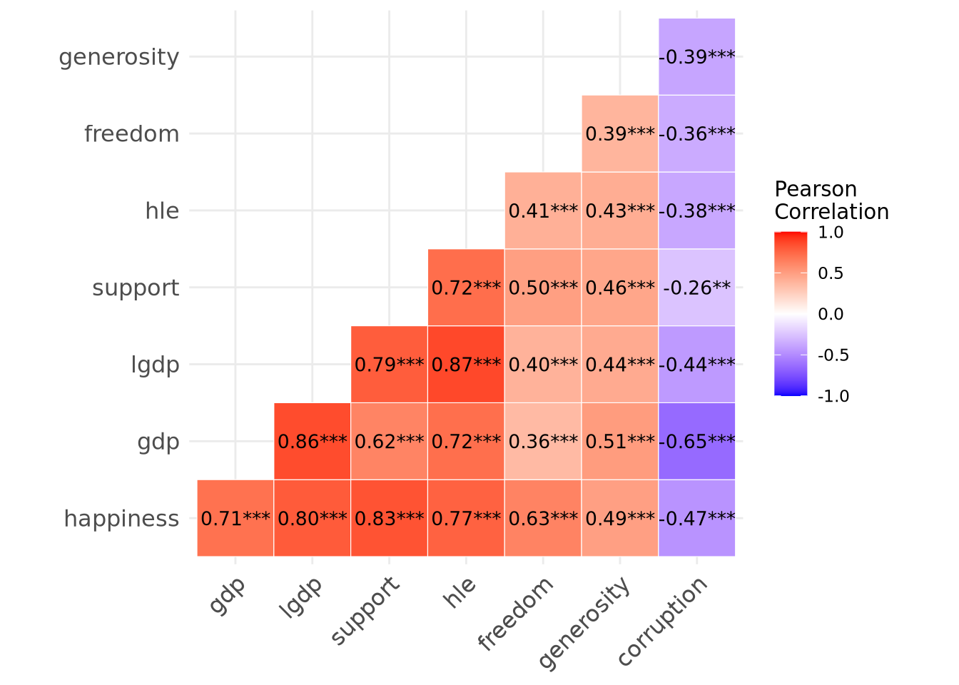
This shows that every variable is correlated with every other variable, sometimes positively or sometimes negatively, but often with a high correlation. The *** indicate that all correlations are significant at \(p < 0.001\). Looking at the last row in particular shows that happiness is significantly correlated with all the other predictors, and the rest of the plot shows that all those predictors are correlated with one another too.
While the pairwise correlations are informative, they only show the linear relationship between two variables considered in isolation. They cannot reveal how much of the variation in happiness can be explained by all predictors acting together. They also cannot show what each predictor contributes beyond the others. The strong correlation between, for example, happiness and support might simply reflect that perceived social support is related to income, health, and other factors that themselves relate to life satisfaction. That single correlation number blends the part of the association specific to social support with the part it shares through those other predictors, and it cannot separate the two. A multiple linear regression model can make that separation. The overall model tells us how much of the total variation in happiness the whole set of predictors accounts for. Each regression coefficient shows how much happiness is expected to change, on average, when one predictor changes by one unit while the others are held constant, thereby showing that predictor’s unique contribution.
8.2 Statistical model
The statistical model in multiple linear regression is an extension of that of the simple linear regression. In simple linear regression, see Section 7.2, we said that the outcome variable is assumed to be normally distributed around a mean that varies as a linear function of its one predictor. In multiple linear regression, the outcome variable is again assumed to be normally distributed, but now the mean of that normal distribution varies as a linear function of more than one predictor. Put another way, multiple linear regression assumes that we have a normal distribution over some variable, with a fixed but unknown width, whose mean is changing whenever the values of any of its predictor variables change. Just like in simple linear regression, this does not mean that we assume that there is a normal distribution over the outcome variable overall. Rather, it assumes that there is a conditionally normal distribution; for any combination of values of the predictor variables, there is a normal distribution over the outcome variable.
In more detail, we denote the \(n\) observations of the outcome variable by \(y_1, y_2 \ldots y_i \ldots y_n\), just as we did with simple linear regression. We will denote the corresponding set of \(K\) predictor variables by \(\vec{x}_i\): \[ \vec{x}_i = [x_{1i}, x_{2i} \ldots x_{ki} \ldots x_{Ki}]. \] In other words, \(\vec{x}_i\) is the set of values of the \(K\) predictor variables at observation \(i\), where \(K\) simply represents the total number of predictors in the model. For example, \(x_{1i}\) is the value of the first predictor, \(x_{2i}\) is the value of the second, \(x_{ki}\) being the value of the predictor \(k\), and so on. (The arrow notation \(\vec{\phantom{x}}\) is commonly used to indicate that a variable represents a vector or array of values — in this context, a list of numbers such as all the predictor values for a single observation.)
We assume the following relationship between the outcome and explanatory variables: \[ y_i \sim N(\mu_i, \sigma^2),\quad \mu_i = \beta_0 + \sum_{k=1}^K \beta_k x_{ki}. \] We use the \(\sum_{k=1}^K\) notation here because it allows for a compact expression, but it just signifies a sum over the \(K\) predictors. In other words, \[ \beta_0 + \sum_{k=1}^K \beta_k x_{ki} = \beta_0 + \beta_1 x_{1i} + \beta_2 x_{2i} + \ldots \beta_k x_{ki} + \ldots \beta_{K} x_{Ki}. \] Just as was the case in simple linear regression, we can also write this statistical model as follows: \[ y_i = \beta_0 + \sum_{k=1}^K \beta_k x_{ki} + \epsilon_i,\quad \epsilon_i \sim N(0, \sigma^2). \] These two forms are mathematically identical, and each one has its advantages as we discussed in Section 7.2.
However it is formally specified, the statistical model assumes that each observation \(y_i\) is modelled as being drawn from a normal distribution with a standard deviation \(\sigma\) (variance \(\sigma^2\)), whose mean \(\mu_i\) is a linear function of the \(K\) predictor variables \(\vec{x}_i\). The linear relationship implies that for every combination of values of the \(K\) predictor variables, there is a corresponding mean to the normal distribution over the outcome. If we change any predictor variable \(k\) by some amount \(\delta_k\), the corresponding mean of the normal distribution over the outcome variable will change by exactly \(\beta_k \delta_k\). This holds no matter what the values of all the predictors are, and for every predictor variable. This is the defining property of a linear equation, and is particularly important when interpreting the meaning of the coefficients in the fitted multiple regression model, as we will see.
8.3 Estimation, model fitting, and inference
In general, multiple linear regression with \(K\) predictor variables involves \(K + 2\) parameters whose values must be inferred. These include the coefficients for each of the \(K\) predictors, the intercept term, and the standard deviation \(\sigma\). Inference about this parameter set proceeds exactly as in the simple linear regression case (see Section 7.3):
- We use estimator formulas to estimate the parameter values. These estimates are essentially our best guesses about the true parameter values.
- We derive the sampling distribution of these estimates for different hypothetical values of the parameters. In other words, we determine the distribution of possible estimate values that could occur in principle if the true value of an unknown parameter had some hypothesised value.
- Once we know these sampling distributions, we can test hypotheses, obtain p-values, and calculate confidence intervals.
In the case of simple linear regression, the estimates of the coefficients of the linear equation were those values that minimise the line of best fit, defined by minimising the sum of squared residuals, also known as residual sum of squares (RSS). In multiple linear regression, the estimates are also those values that minimise the RSS. In other words, the estimates of the coefficients, denoted by \(\hat{\beta}_0, \hat{\beta}_1, \ldots \hat{\beta}_k \ldots \hat{\beta}_K\), are those that minimise the following sum: \[ \textrm{RSS} = \sum_{i=1}^n \hat{\epsilon}_i^2 = \sum_{i=1}^n (y_i - \hat{\mu}_i)^2, \quad\text{where }\hat{\mu}_i = \hat{\beta}_0 + \sum_{k=1}^K \hat{\beta}_k x_{ki}. \] In other words, \(\hat{\mu}_i\) is the predicted mean of the outcome variable corresponding to point \(\vec{x}_i\) when the coefficients are \(\hat{\beta}_0, \hat{\beta}_1, \ldots \hat{\beta}_k \ldots \hat{\beta}_K\). The \(\hat{\epsilon}_i = y_i - \hat{\mu}_i\) is the residual for observation \(i\): the difference between the observed value of the outcome variable and the mean predicted by the model.
Note 8.1: Hyperplane of best fit
In simple linear regression, we said that \(\hat{\beta}_0\) and \(\hat{\beta}_1\), the values of the intercept and slope that minimised the RSS, defined the line of best fit. In the case of multiple linear regression, the linear equation no longer defines a line because there is more than one predictor. If there were exactly two predictors, the linear equation would be \(\mu_i = \beta_0 + \beta_1 x_{1i} + \beta_2 x_{2i}\). In this case, the coefficients that minimise the RSS would be \(\hat{\beta}_0, \hat{\beta}_1, \hat{\beta}_2\). These define the plane of best fit, with a plane being a perfectly flat surface extending infinitely in all directions, like an infinitely large, perfectly flat sheet of paper. When we have \(K > 2\) predictors, the \(K+1\) coefficients that minimise RSS, \(\hat{\beta}_0, \hat{\beta}_1, \ldots \hat{\beta}_k \ldots \hat{\beta}_K\), now define a hyperplane of best fit, which is a generalisation of the concept of plane to higher dimensions.
Don’t worry if you can’t visualise a hyperplane; nobody can. Our brains can handle lines and planes, but visualising higher-dimensional ‘flat surfaces’ is beyond human capability. Mathematically, we know what they are, but we work with them through equations rather than mental pictures.
In the case of simple linear regression, there was a relatively manageable formula to calculate the estimates of the intercept and slope. For multiple regression, the corresponding formulas are quite compact to write but can only be done using matrix notation and operations. A matrix is simply a rectangular array of numbers and there are special rules for doing mathematical operations like multiplication with these arrays. Explaining matrices and their operations would take us far beyond the mathematical scope of this book. The key point is that while simple linear regression has relatively manageable formulas that you could in principle work through by hand, multiple regression requires these more sophisticated mathematical tools. The good news is that languages like R have all these tools built in and can do these required calculations in milliseconds or even microseconds (Note 8.2).
Note 8.2: How computers have revolutionised statistics
Multiple regression is essentially unthinkable to do by hand. Even for small datasets like this chapter’s example, estimating coefficients requires over 10,000 arithmetic calculations - potentially 10 hours of error-prone work with paper and calculator.
Modern computers perform these calculations in milliseconds with essentially zero error. This represents a speed increase of billions of times compared to hand calculation, fundamentally transforming statistical practice by making previously impossible analyses routine.
Once we have the estimates of the coefficients, we can then calculate the estimate of the residual standard deviation, which we denote by \(\hat{\sigma}\), as follows: \[ \hat{\sigma} = \sqrt{\frac{\textrm{RSS}}{n-K-1}}. \] This is, in fact, the same formula that was used in the case of simple linear regression. In that case, the denominator was \(n-2\), but that is exactly \(n-K-1\) in the case of simple linear regression where \(K=1\).
Having obtained the estimates of the parameters, we can use other theoretical results to derive their sampling distributions. These results allow us to work out the standard errors, which are the standard deviations of the sampling distributions, and with the standard errors, we can calculate test statistics for any hypothetical values of the parameters. For the coefficients, we can test any hypothesis about its true value using the following result, which is also used in simple linear regression: \[ \frac{\hat\beta_k-\beta_k}{\operatorname{SE}(\hat\beta_k)} \sim\textrm{Student-t}(n-K-1). \] In other words, if we hypothesise that the true value of coefficient \(k\) is \(\beta_k\), the sampling distribution of the t-statistic \((\hat\beta_k-\beta_k)/\operatorname{SE}(\hat\beta_k)\) has a t-distribution with \(n-K-1\). Using the general logic of hypothesis testing that we followed in Chapter 4, Chapter 6, and Chapter 7, we can calculate p-values for any hypothesised value of any coefficient. As always, this p-value effectively quantifies the degree of compatibility between the data and the hypothesised value of the coefficient; the lower the p-value, the less evidence there is for the hypothesis.
Likewise, confidence intervals follow the same general logic as was covered in Chapter 4, Chapter 6, and Chapter 7. In particular, the \(\gamma\), such as \(\gamma=0.95\), confidence interval for any coefficient is its estimate plus or minus a \(t\) critical value (see Note 6.3), \(T(\gamma,n-K-1)\), times its standard error: \[ \hat\beta_j \pm T(\gamma, n-K-1) \operatorname{SE}(\hat\beta_j). \] This is exactly the same general result as was used for confidence intervals in simple linear regression, but there the degrees of freedom were written as \(n-2\) because \(K=1\) in that case.
8.4 Using lm()
The analysis we will conduct has happiness as the outcome variable. We can in principle use all other variables other than country as predictors. However, because gdp and lgdp are highly similar to one another, and both measure the same thing (the country’s average per capita income), we should use just one of them. For reasons discussed in Section 7.1, where we used the whr2025 dataset, the lgdp variable is a better choice if we assume linearity.
To perform a multiple linear regression in R, we use lm(), just as we did with simple linear regression. For example, to do the multiple linear regression with the whr2024 dataset, with happiness as the outcome variable and lgdp, support, hle, freedom, generosity, and corruption as predictors, we do the following:
M_8_1 <- lm(happiness ~ lgdp + support + hle + freedom + generosity + corruption,
            data = whr2024)
Note how this is exactly what we did when doing simple linear regression with the exception that there is now more than one predictor variable on the right hand side of the ~ in the R formula, and those predictors are specified with + between them. This is the general R formula for regression analysis:
outcome_variable ~ predictor_1 + predictor_2 + ... + predictor_K.Just as we did with simple linear regression, the usual procedure to examine the main results of the analysis is to use summary():
summary(M_8_1)
Call:
lm(formula = happiness ~ lgdp + support + hle + freedom + generosity +
    corruption, data = whr2024)

Residuals:
    Min      1Q  Median      3Q     Max
-1.5699 -0.2506  0.0651  0.3181  1.1344

Coefficients:
            Estimate Std. Error t value Pr(>|t|)
(Intercept) -2.29158    0.67310  -3.405 0.000893 ***
lgdp         0.32800    0.21389   1.534 0.127694
support      3.78694    0.61173   6.191 8.05e-09 ***
hle          0.03580    0.01429   2.505 0.013560 *
freedom      2.29692    0.45994   4.994 1.96e-06 ***
generosity   0.10107    0.31366   0.322 0.747813
corruption  -0.91498    0.31008  -2.951 0.003791 **
---
Signif. codes:  0 '***' 0.001 '**' 0.01 '*' 0.05 '.' 0.1 ' ' 1

Residual standard error: 0.5066 on 124 degrees of freedom
Multiple R-squared:  0.8262,    Adjusted R-squared:  0.8177
F-statistic: 98.22 on 6 and 124 DF,  p-value: < 2.2e-16
The output here is just like it was with the simple linear regression, except that now there are more coefficients in the Coefficients: table.
Just as we did in Section 7.4, we can break this output down into its parts.
- Residuals
- The five number residuals summary provides a quick diagnostic check on the distribution of residuals. Ideally the median should be close to 0 and the lower half (Min, 1Q) should mirror the upper half (3Q, Max) so the residuals look roughly symmetric with no huge outliers. Here the median is relatively close to zero, the 1st and 3rd quartiles are about the same distance from zero, and the most negative residual (-1.57) is only a little larger in magnitude than the most positive one (1.13). That pattern is consistent with an approximately normal, symmetric error distribution.
- Coefficients
- As always, the coefficients table has four columns:
Estimate: This is \(\hat\beta_k\), the estimate of the coefficient. For slope coefficients, it is the expected change in the outcome for a one-unit change in that predictor while holding the other predictors fixed. Note how this is subtly but importantly different to the meaning of a coefficient’s value in simple linear regression.Std. Error: This is the estimated standard deviation of the sampling distribution of \(\hat\beta_k\). Larger values mean more sampling noise, which in turn entails higher p-values for the null hypothesis, and wider confidence intervals.t value: The t-statistic \(\hat\beta_k/\operatorname{SE}(\hat\beta_k)\) for the null hypothesis that \(\beta_k=0\). Under the null hypothesis, this t-statistic follows a \(t\) distribution with \(n-K-1\) degrees of freedom.Pr(>|t|): The p-value associated with the t-statistic. Low values, \(p < 0.05\), indicate that the data is not compatible with the null hypothesis for that coefficient.
Going through each row in the coefficients table, the interpretation is as follows:
(Intercept): This is the predicted average ofhappinesswhen every predictor equals zero. The intercept term is needed to anchor the plane but is not of substantive interest here because values of zero for most predictors do not have any real meaning.lgdp: A one-unit rise in base-10 log-GDP (a 10-fold increase in GDP) is associated with a 0.328 increase inhappiness, after accounting for all other variables. However, the p-value for the null hypothesis is p = 0.128. As such, we cannot rule out a partial effect of zero.support: All else being equal, increasing perceived social support by one unit raises the predicted mean ofhappinessby 3.79 units. Becausesupportrepresents the proportion of respondents who say they can rely on the social support of family and friends, a one unit change means going from 0% to 100%, which is an unrealistically large change given that no country is as low as 0% or as high as 100%. A more meaningful unit of change might be a 10% (0.1) change insupport. This corresponds to a \(0.1 \times 3.79\), or 0.379, in the predicted averagehappiness. The null hypothesis p-value is p < 0.001, which is a significant result, or low degree of support for the null.hle: Each extra healthy-life-expectancy year increases averagehappinessby roughly 0.0358 points, assuming all other factors are held constant. The null hypothesis p-value is p = 0.0136, which is significant.freedom: Given thatfreedomalso represents a proportion, it is more meaningful to talk about a change like 10%, as we did forsupport. A 10% change infreedomcorresponds to a \(0.1 \times 0.0358\), or 0.23, in the predicted averagehappiness. The p-value for the null is p < 0.001, which is highly significant.generosity: The coefficient is low, 0.101, and the p-value for the null is high, p = 0.748, indicating no discernible association between national generosity scores and average life satisfaction once the other predictors are included.corruption: This variable is also a proportion, so it is meaningful to consider changes of around 10%. A 10% rise in perceived corruption increases averagehappinessby about -0.915 points (in other words, higher corruption leads to lower life satisfaction), controlling for the other variables. The p-value for the null is highly significant, p = 0.00379.
- Model summary
-
The final section of the
summary()output is usually referred to as the model summary. This always contains three lines. We will discuss the results on the second and third lines (Multiple R-squared,Adjusted R-squared,F-statistic) in Section 8.6. The first line provides the so-called residual standard error value. As mentioned in Chapter 7, the term residual standard error is a misnomer. This is in fact \(\hat{\sigma}\), the estimate of the residual standard deviation \(\sigma\). This tells us that for any possible combination of the predictors, there is a normal distribution overhappinesswhose standard deviation is estimated to be 0.507. The degrees of freedom listed on that line is \(n - K - 1\), which is the degrees of freedom used for calculating all p-values for the coefficients’ hypothesis tests, and also for calculating their confidence intervals.
As discussed in the case of simple linear regression, summary() does not return the confidence intervals for the coefficients. These can be obtained using the confint() function, which by default gives the 95% confidence interval:
confint(M_8_1) 2.5 % 97.5 %
(Intercept) -3.623829943 -0.95933943
lgdp -0.095341898 0.75135095
support 2.576159973 4.99772241
hle 0.007507643 0.06409123
freedom 1.386574804 3.20726377
generosity -0.519752688 0.72190257
corruption -1.528709896 -0.30124688These intervals give the ranges of coefficient values that are compatible with the data; those values that would not be rejected at the 0.05 level of significance. As has to be the case, we see that for all those coefficients whose null hypothesis p-values were greater than 0.05, the confidence interval extends from a negative to a positive value. In other words, for each of these coefficients, the null value of 0 is compatible with the data. For all other coefficients, the confidence interval is either all negative or all positive. For example, the 95% confidence interval for hle is 0.008, 0.064. This means that a true value of the coefficient anywhere from 0.008 to 0.064 is compatible with the data.
As also discussed in the case of simple linear regression, the tidy() function from the broom package provides the coefficients and the confidence intervals as a tibble:
tidy(M_8_1, conf.int = TRUE)# A tibble: 7 × 7
term estimate std.error statistic p.value conf.low conf.high
<chr> <dbl> <dbl> <dbl> <dbl> <dbl> <dbl>
1 (Intercept) -2.29 0.673 -3.40 0.000893 -3.62 -0.959
2 lgdp 0.328 0.214 1.53 0.128 -0.0953 0.751
3 support 3.79 0.612 6.19 0.00000000805 2.58 5.00
4 hle 0.0358 0.0143 2.50 0.0136 0.00751 0.0641
5 freedom 2.30 0.460 4.99 0.00000196 1.39 3.21
6 generosity 0.101 0.314 0.322 0.748 -0.520 0.722
7 corruption -0.915 0.310 -2.95 0.00379 -1.53 -0.301 This is the same information as before, but the format is more useful for some purposes.
8.4.1 Standardised coefficients
The meaning of a coefficient in a multiple linear regression is the change in the mean of the outcome variable for a one unit change in the predictor, assuming all other variables are held constant. We therefore interpret coefficients in terms of their original measurement units, which is essential for concrete interpretations. For example, the coefficient for hle is 0.0358 and this means that each extra healthy-life-expectancy year increases happiness by 0.0358 points. But this interpretation also means that the value of a coefficient says as much about the units chosen as about the strength of association. For example, a variable recorded in tens of thousands of dollars will yield a slope one-tenth the size of the same variable recorded in thousands, even though the substantive effect is identical. This makes the coefficients difficult to compare with one another or across studies.
In order to facilitate comparison of coefficients, we can use standardised coefficients. These can be obtained by re-scaling all predictors and the outcome variable to have a mean of zero and a standard deviation of 1. As a consequence, every predictor and the outcome variable are on the same metric: a unit change on each variable is a change of one standard deviation. A standardised coefficient tells us the change in standard deviations of the outcome variable for a one standard deviation change of the predictor variable.
In order to obtain standardised coefficients, we will use the re_scale() function from sgsur to re-scale all variables:
M_8_1s <- lm(happiness ~ lgdp + support + hle + freedom + generosity + corruption,
             data = re_scale(whr2024))
In the following, we use tidy() as we did above to obtain the standardised coefficients and their corresponding inferential statistics including confidence intervals:
tidy(M_8_1s, conf.int = TRUE)# A tibble: 7 × 7
term estimate std.error statistic p.value conf.low conf.high
<chr> <dbl> <dbl> <dbl> <dbl> <dbl> <dbl>
1 (Intercept) 3.72e-17 0.0373 9.97e-16 1.000 -0.0738 0.0738
2 lgdp 1.39e- 1 0.0909 1.53e+ 0 0.128 -0.0405 0.319
3 support 4.26e- 1 0.0687 6.19e+ 0 0.00000000805 0.289 0.562
4 hle 1.92e- 1 0.0767 2.50e+ 0 0.0136 0.0403 0.344
5 freedom 2.29e- 1 0.0458 4.99e+ 0 0.00000196 0.138 0.319
6 generosity 1.45e- 2 0.0449 3.22e- 1 0.748 -0.0744 0.103
7 corruption -1.34e- 1 0.0456 -2.95e+ 0 0.00379 -0.225 -0.0443The only problem with this output is due to the fact that the intercept term is effectively zero (this is always the case when all variables are standardised) but represented by a tiny number, which makes all other variables shown in scientific notation. The easiest remedy is to remove the intercept’s row with filter() (see Section 5.5):
tidy(M_8_1s, conf.int = TRUE) |>
  filter(term != '(Intercept)')
# A tibble: 6 × 7
term estimate std.error statistic p.value conf.low conf.high
<chr> <dbl> <dbl> <dbl> <dbl> <dbl> <dbl>
1 lgdp 0.139 0.0909 1.53 0.128 -0.0405 0.319
2 support 0.426 0.0687 6.19 0.00000000805 0.289 0.562
3 hle 0.192 0.0767 2.50 0.0136 0.0403 0.344
4 freedom 0.229 0.0458 4.99 0.00000196 0.138 0.319
5 generosity 0.0145 0.0449 0.322 0.748 -0.0744 0.103
6 corruption -0.134 0.0456 -2.95 0.00379 -0.225 -0.0443This allows us to compare across the predictors more easily. For example, a one standard deviation change in support leads to a 0.43 standard deviation change in happiness. By contrast, a one standard deviation change in hle leads to a 0.19 standard deviation change in happiness. It’s important to note here that rescaling does not affect the fit of the model or its p-values. The relationships among variables remain unchanged — standardisation simply rescales the variables so that the coefficients are expressed in standard deviation units rather than in their original measurement scales.
8.5 Covariates and statistical control
In model M_8_1, the lgdp variable does not tell us much about happiness. Let’s look at the relevant coefficients table row returned by tidy():
tidy(M_8_1, conf.int = T) |> filter(term == 'lgdp')# A tibble: 1 × 7
term estimate std.error statistic p.value conf.low conf.high
<chr> <dbl> <dbl> <dbl> <dbl> <dbl> <dbl>
1 lgdp 0.328 0.214 1.53 0.128 -0.0953 0.751The coefficient estimate is 0.328, with a confidence interval between -0.095 and 0.751. Because this interval includes zero, the data are compatible with no effect of lgdp once other variables are controlled for (that is, the population value of the coefficient could be 0) , meaning the p-value is non-significant (p = 0.128). This contrasts with what we found in model M_7_1, the simple linear regression model discussed in Chapter 7. There, we used a similar dataset (M_7_1 used whr2025, the World Happiness Report 2025 edition), and found the lgdp coefficient had an estimate of 1.86, with a confidence interval between 1.631 and 2.089, and a highly significant p-value (p < 0.001).
Despite very similar datasets and variables, the results with respect to the role of lgdp on happiness are very different. To confirm that this is not because of something hidden in the datasets, let us perform a simple linear regression with happiness as outcome and lgdp as the predictor using the same whr2024 dataset that we used with M_8_1:
M_8_2 <- lm(happiness ~ lgdp, data = whr2024)Focusing on the lgdp coefficient results, we have:
tidy(M_8_2, conf.int = T) |> filter(term == 'lgdp')# A tibble: 1 × 7
term estimate std.error statistic p.value conf.low conf.high
<chr> <dbl> <dbl> <dbl> <dbl> <dbl> <dbl>
1 lgdp 1.88 0.124 15.1 2.18e-30 1.64 2.13This is very similar to what we found with M_7_1: the coefficient has an estimate of 1.882, with a confidence interval between 1.636 and 2.128, a highly significant p-value (p < 0.001).
Why is it that lgdp appears to be a very important predictor of happiness according to model M_8_2 (and M_7_1), but a weak or negligible predictor according to M_8_1? Model M_8_1 and M_8_2 seem to conflict, at least with respect to the role of lgdp on happiness. If so, which model is correct? Well, both are correct. They are different models and tell us different things. They do not conflict or contradict one another.
The meaning of any predictor’s coefficient in any multiple regression model is the change in the average value of the outcome for a one unit change of the predictor assuming all other variables are held constant. To understand this with respect to M_8_1 and lgdp, imagine we have two sets of countries that are identical in all respects except in their per capita GDP. They have the same levels of hle, support, corruption, and so on. According to M_8_1, when we hold these other factors constant, countries that differ in lgdp do not differ much, or at all, in their average happiness.
By contrast, in a simple linear regression nothing else is held fixed, so lgdp effectively stands in for every pathway by which GDP and the things correlated with GDP can influence happiness. For example, wealthy countries tend to have longer healthy life expectancy, stronger social-support networks, more personal freedom and, in many cases, lower corruption. All of these other factors increase happiness, but because we have just a single predictor, the coefficient effectively stands for the joint contribution of GDP and everything correlated with GDP.
Once the model explicitly includes support, hle, freedom, generosity, and corruption, the contribution of each of those variables is accounted for individually, rather than being rolled into lgdp’s contribution. More precisely, the lgdp coefficient is now estimated only from the residual part of income that is independent of the other five predictors. Conceptually, it’s as if we first modelled lgdp using the other predictors and then examined how the remaining residual variation in lgdp relates to happiness. Because these other variables already explain most of the useful variation in lgdp, that residual is small and so only weakly related to happiness. Consequently \(\hat\beta_{\text{lgdp}}\) shrinks to about 0.3 and its confidence interval covers zero.
Another way to phrase the result is in terms of partial versus total association. The simple regression slope between lgdp and happiness measures the total association between lgdp and happiness, including every indirect path through other country characteristics. The multiple regression slope measures the partial association, namely the relationship that remains after removing any part that is predictable from the covariates. If those covariates account for nearly all systematic differences in happiness that coincide with differences in income, the partial effect of lgdp must be small.
These regression concepts are related to the concept of correlation and partial correlation. We saw in Chapter 3, that we can calculate the Pearson correlation between lgdp and happiness as follows:
summarise(whr2024, corr = cor(lgdp, happiness))# A tibble: 1 × 1
corr
<dbl>
1 0.800The partial correlation between lgdp and happiness, after we partial out the effects of support, hle, freedom, generosity, and corruption, can be calculated using the partial_corr() function from sgsur:
partial_corr(lgdp, happiness,
             controls = c(support, hle, freedom, generosity, corruption),
             data = whr2024)
# A tibble: 1 × 5
estimate statistic p_value n gn
<dbl> <dbl> <dbl> <int> <dbl>
1 0.136 1.53 0.128 131 5Technically, this partial correlation is the correlation between the residuals of two models. One model has happiness as the outcome and support, hle, freedom, generosity, and corruption as predictors. The other model has lgdp as the outcome and again support, hle, freedom, generosity, and corruption as predictors. In other words, it isolates the association between lgdp and happiness after the effects of all other predictors have been removed from both variables. It compares what is unique to lgdp with what is unique to happiness, and it informs about how much happiness would change when lgdp changes and nothing else in the model changes.
Thus, M_8_1 does not contradict M_8_2; it refines it. When we ask the general question, “Are richer countries happier on average?” the answer from M_8_2 is an emphatic “yes,” but that reflects the set of advantages that are associated with higher national income rather than money per se. As such, when we ask, “Are richer countries happier everything else being equal?”, the answer from M_8_1 is “not much.” This confirms that it is not income per se that matters for happiness, but the fact that higher income leads to increases in other factors that in turn leads to higher happiness.
8.6 Model evaluation
Once we have fitted a multiple-regression model, we can measure its goodness of fit. This can be measured by how close each predicted mean of the outcome \(\hat{\mu}_i\) is to the observed value of the outcome \(y_i\). This is given by the residual sum of squares (RSS), which we’ve already seen is defined as follows: \[ \textrm{RSS} = \sum_{i=1}^n \hat{\epsilon}_i^2 = \sum_{i=1}^n (y_i - \hat{\mu}_i)^2. \] The smaller the RSS, the closer the model fits the data, so in that sense RSS is a measure of lack of fit.
Because RSS is expressed in the units of the outcome variable and also grows with the sample size, it is hard to interpret on its own, so we can scale it by comparing it with the total sum of squares (TSS): \[ \textrm{TSS} = \sum_{i=1}^n (y_i-\bar y)^2. \] TSS represents the total variability, or overall spread, in the outcome variable. It is, in fact, just the variance of \(y\) multiplied by \(n-1\).
Note how the two equations are structurally very similar: both compare each observed value \(y_i\) with a reference point and then square and sum the differences. In the case of TSS, the reference point is the overall mean \(\bar{y}\), while for RSS it is the model’s predicted mean \(\hat{\mu}_i\) for that specific observation, based on its predictor values. TSS therefore captures the total variability of the data around their mean, whereas RSS captures the remaining, unexplained variability of the data around each data point’s predicted value.
The proportion RSS/TSS tells us how much of the total variability in the data is due to randomness or unexplained noise. By contrast, the proportion of the total variability that is not due to unexplained noise is 1 minus RSS/TSS. This is known as the \(R^2\) value, which is sometimes also known as the coefficient of determination: \[ R^2 = 1 - \frac{\textrm{RSS}}{\textrm{TSS}}. \]
In normal linear models, TSS = ESS + RSS, where ESS is the explained sum of squares, which is the variability in the predicted means of the outcome variable: \[ \underbrace{\sum_{i=1}^n (y_i-\bar{y})^2}_{\text{TSS}} = \underbrace{\sum_{i=1}^n (\hat{\mu}_i - \bar{y})^2}_{\text{ESS}} + \underbrace{\sum_{i=1}^n (y_i - \hat{\mu}_i)^2}_{\text{RSS}}. \] Because of this, \(R^2\) is also defined as \[ R^2 = \frac{\textrm{ESS}}{\textrm{TSS}}. \]
More concretely, \(R^2\) represents the proportion of variability in the outcome that arises from the natural variability in the predictor variables, as opposed to random noise or measurement error. Because the outcome variable changes systematically as the predictor variables change, we can attribute some of the total variability in the outcome to the fact that the predictor variables themselves vary naturally across observations. The coefficient \(R^2\) quantifies this relationship by measuring how much of the outcome’s variability can be traced back to the systematic patterns associated with the predictor variables, rather than to unexplained random fluctuations.
\(R^2\) must be a value between 0 and 1. A value at or very close to 0 means that there is no systematic relationship between the set of predictors and the outcome. A value at or very close to 1 means that the predictor can perfectly, or almost perfectly, predict the value of the outcome.
There are no universally agreed upon numerical cut-offs that statisticians accept as “low”, “medium”, or “high” \(R^2\) values across every kind of study, because the statistic is unavoidably tied to the nature of the outcome, the design, and the amount of uncontrollable noise in a given context. While a low \(R^2\) value does mean that a low proportion of the variability can be explained by the predictor, and so most variability is unexplained, this does not necessarily mean the model is poor or not useful. It just means that there are many other as yet unaccounted for factors that can explain variability in the outcome.
For lm() models, the value of \(R^2\) is given in the second to last line of the summary() output, labelled Multiple R-squared:. We can also obtain it using the get_rsq() function from sgsur, which includes its 95% confidence interval:
get_rsq(M_8_1)# A tibble: 1 × 3
rsq ci_low ci_high
<dbl> <dbl> <dbl>
1 0.826 0.752 0.868By the standards in social science, this is a high value. It therefore means that a large proportion of the variability of happiness across countries can be accounted for by the natural variation in the predictors lgdp, support, hle, etc.
8.6.1 Overall model null hypothesis
The coefficient of determination can also be used for hypothesis testing purposes. A test that \(R^2=0\) is mathematically identical to testing whether all slope coefficients equal zero, that is, whether \(\beta_1 = \beta_2 = \ldots = \beta_k = \ldots = \beta_K = 0\). In other words, it is the hypothesis that, for all \(K\) predictors, the null hypothesis \(\beta_k = 0\) is true.
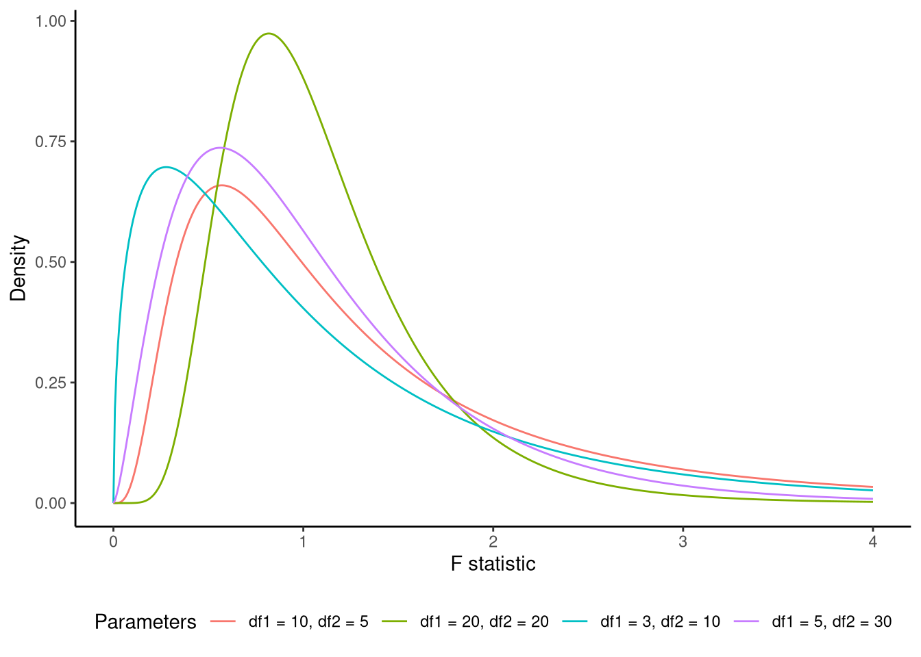
When this overall null hypothesis holds true, the following test statistic, known as the F-statistic, follows an F distribution: \[ \underbrace{\frac{\text{ESS}/K}{\textrm{RSS}/(n-K-1)}}_{\textrm{F-statistic}} \sim \textrm{F}_{(K,n-K-1)}. \] An F distribution is a continuous probability distribution over non-negative values (see Figure 8.2 for examples). It has two parameters, which are known as its degrees of freedom. The first parameter is known as its numerator degrees of freedom, and has a value of \(K\), and the second parameter is known as the denominator degrees of freedom, and has a value of \(n - K - 1\). Because it describes how variance ratios behave under the null hypothesis, it serves as the reference distribution for F-tests in regression, ANOVA, and many other procedures that compare explained to unexplained variation.
Following standard hypothesis testing procedures, if the F-statistic exceeds a critical threshold (the value below which 95% of the F distribution’s mass lies), we may reject the null hypothesis that \(R^2=0\) and that the null hypothesis is simultaneously true for all predictors. This would provide evidence that our model explains a statistically significant portion of the variation in the dependent variable.
From the lm() model, we can obtain the null hypothesis F-statistic, its two degrees of freedom, and its p-value from the last line of the summary() output. These values can also be obtained using get_fstat() from sgsur:
get_fstat(M_8_1)# A tibble: 1 × 4
fstat num_df den_df p_value
<dbl> <dbl> <int> <dbl>
1 98.2 6 124 1.07e-44We would write this as \(F(6, 124) = 98.2\), \(p < 0.001\). Because the p-value is very low, we can reject the overall model null hypothesis. In other words, we have sufficient evidence to conclude that at least one of the predictors contributes to explaining variation in the outcome, meaning that the model as a whole provides a significantly better fit than a model with no predictors.
8.6.2 Adjusted \(R^2\)
\(R^2\) always increases, or at best stays the same, whenever you add another predictor variable, even if that new variable is just random noise. As a result, it is a biased and overly optimistic estimate of how much variance can be explained in the population.
Adjusted \(R^2\) fixes that bias by scaling the unexplained-variance term by an adjustment factor. Formally it replaces \(1 - \textrm{RSS}/\textrm{TSS}\) with \[ 1 - \frac{\textrm{RSS}/(n - K - 1)}{\textrm{TSS}/(n - 1)}. \]
If any new variable is useless, the statistic drops, giving you a signal to keep the simpler model. Under the classical linear-model assumptions (discussed in Section 7.6 and Section 8.10 below) this adjustment also makes the statistic an unbiased estimator of the population proportion of variance explained, which is especially helpful in small samples.
The adjusted \(R^2\) value is also available on the second to last line of the summary() output, labelled as Adjusted R-squared:. It may also be obtained, along with its confidence interval, using the get_adjrsq() function from sgsur:
get_adjrsq(M_8_1)# A tibble: 1 × 3
adj_rsq ci_low ci_high
<dbl> <dbl> <dbl>
1 0.818 0.740 0.8618.7 Nested model comparison
The concept of nested models is a cornerstone of statistical modelling and model comparison procedures. In general, a nested model relationship exists when one model can be viewed as a special case or restricted version of another, larger model. In multiple linear regression, if we have two models, \(M_0\) and \(M_1\), both with the same outcome variable, but the predictors of \(M_0\) are a subset of those of \(M_1\), then we say that \(M_0\) is nested in \(M_1\). In this case, \(M_0\) is often said to be the reduced or null model, with \(M_1\) being the full model.
As a concrete example, the following M_8_3 model is nested in M_8_1 given that it uses a subset of M_8_1’s six predictors:
M_8_3 <- lm(happiness ~ lgdp + support + hle, data = whr2024)To make the following descriptions clearer, let’s create two new model objects, M_0 and M_1, with M_0 pointing to the model M_8_3 and M_1 pointing to the model in M_8_1.
M_0 <- M_8_3
M_1 <- M_8_1
Now we can refer to the reduced model as M_0 and the full model as M_1 in the generic nesting notation, but we have not altered or discarded the original M_8_3 and M_8_1 objects.
When we have two nested normal linear models, we can quantify their relative performance by examining their residual sums of squares. The residual sum of squares for each model, denoted as \(\text{RSS}_0\) and \(\text{RSS}_1\) respectively, measures the total amount of variation in the outcome variable that remains unexplained after fitting each model. We can easily extract the residual sum of squares for an lm() model using get_rss() from sgsur.
RSS_0 <- get_rss(M_0) # RSS of the reduced model
RSS_1 <- get_rss(M_1) # RSS of the full model

c(RSS_0, RSS_1)
[1] 44.50838 31.82902A fundamental property of nested model comparisons is that \(\text{RSS}_0\) will always be greater than or equal to \(\text{RSS}_1\). This inequality follows logically from the nesting relationship: since \(M_1\) contains all the parameters of \(M_0\) plus additional parameters, it has at least as much flexibility to fit the data as \(M_0\), and potentially more. The additional parameters in \(M_1\) can only improve the fit (or leave it unchanged if the additional parameters have no predictive value), never make it worse.
A core quantity of interest in nested model comparison is the proportional increase in error when we move from the more complex model \(M_1\) to the simpler model \(M_0\). This can be expressed mathematically as: \[ \begin{aligned} \text{proportional increase in error (PIE)}&= \frac{\text{change in error (from $M_0$ to $M_1$)}}{\text{minimal error}} \\ \\ &= \frac{\text{RSS}_0 - \text{RSS}_1}{\text{RSS}_1} \end{aligned} \] This ratio captures the relative cost, in terms of model fit, of adopting the simpler model instead of the more complex one.
For M_0 and M_1, the proportional increase in error is as follows:
(RSS_0 - RSS_1)/RSS_1[1] 0.3983582This result indicates that \(\text{RSS}_0\) is approximately 1.4 times greater than \(\text{RSS}_1\). This is because a proportional difference of 0.4 implies a multiplicative ratio of 1 + that value. Said another way, the unexplained variance has decreased by about 40% when moving from model 0 to model 1. This quantifies the cost of omitting the 3 predictors, freedom, generosity, corruption, from M_1.
While the proportional increase in error provides a useful measure of effect size, we need a formal statistical test to determine whether the improvement in fit provided by the more complex model is statistically significant. The F-test accomplishes this by incorporating both the effect size (proportional change in error) and the sample size into a single test statistic.
The F-ratio for comparing nested models is calculated as: \[ \begin{aligned} \textrm{F-statistic} &= \underbrace{\frac{\text{RSS}_0 - \text{RSS}_1}{\text{RSS}_1}}_{\text{effect size}} \times \underbrace{\frac{\text{df}_1}{\text{df}_0 - \text{df}_1}}_{\text{sample size}} \\ &= \frac{(\text{RSS}_0 - \text{RSS}_1)/(\text{df}_0 - \text{df}_1)}{\text{RSS}_1/\text{df}_1}. \end{aligned} \] Here, \(\text{df}_0\) and \(\text{df}_1\) are the degrees of freedom for the residuals in model \(M_1\), calculated by \(n - K_0 -1\) and \(n- K_1 -1\), respectively, where \(n\) is the sample size and \(K_0\) and \(K_1\) are the number of predictor variables (excluding the intercept) in \(M_0\) and \(M_1\). The ratio \(\text{df}_1/(\text{df}_0 - \text{df}_1)\) is described here as a sample-size multiplier, but more precisely it is an information-to-complexity ratio: it expresses how many independent pieces of information remain in the full model for every additional parameter you have introduced when moving from \(M_0\) to \(M_1\). The difference in residual degrees of freedom of the two models (\(\text{df}_0 - \text{df}_1\) = 127 - 124 = 3 = \(K_1 - K_0\)) represents the number of additional parameters in the more complex model.
Under the null hypothesis that the reduced model M_0 fits the data as well as the full model M_1, the F-statistic is distributed as an F statistic (see Figure 8.2) with \(K_0 - K_1\) and \(\text{df}_1\) degrees of freedom. In R, the built-in anova() function will calculate the F-statistic, its numerator and denominator degrees of freedom, and the corresponding p-value:
anova(M_0, M_1)Analysis of Variance Table
Model 1: happiness ~ lgdp + support + hle
Model 2: happiness ~ lgdp + support + hle + freedom + generosity + corruption
Res.Df RSS Df Sum of Sq F Pr(>F)
1 127 44.508
2 124 31.829 3 12.679 16.465 4.557e-09 ***
---
Signif. codes: 0 '***' 0.001 '**' 0.01 '*' 0.05 '.' 0.1 ' ' 1As we did in Section 8.6.1, we write this result as \(F(3, 124 ) = 16.47\), \(p < 0.001\). What this significant result means is that we can reject the hypothesis that M_0 fits the data as well as M_1. This is equivalent to saying that we reject the hypothesis that the 3 predictor variables that are in M_1 and not in M_0, i.e., freedom, generosity, corruption, are all null predictors (their slope coefficients are equal to zero). Rejecting the null hypothesis here necessarily means that M_1 fits the data significantly better than M_0, and so the predictors freedom, generosity, corruption significantly contribute to the predictive power of the model over and above the 3 predictor variables that are in M_0, i.e., lgdp, support, hle.
8.7.1 Model null hypothesis as a model comparison
In Section 8.6.1, we described how to test any model’s overall null hypothesis, which is that \(\beta_1 = \beta_2 = \ldots \beta_K = 0\). When it is true \[ \underbrace{\frac{\text{ESS}/K}{\textrm{RSS}/(n-K-1)}}_{\textrm{F-statistic}} \sim \textrm{F}_{(K,n-K-1)}. \]
This F-statistic is exactly the F-statistic we would obtain if we compare a linear regression model with a model with no predictors (see Note 8.3).
Note 8.3: Model null hypothesis F-test
For any linear regression model M_1, its overall null hypothesis is \[
\text{F-statistic} = \frac{\text{ESS}_1/K_1}{\textrm{RSS}_1/(n-K_1-1)},
\] where \(\text{ESS}_1\) and \(\text{RSS}_1\) are M_1’s explained and residual sum of squares, respectively, and \(K_1\) is M_1’s number of predictor variables.
The F-statistic we used for nested model comparison of M_0 and M_1 is \[
\begin{aligned}
\text{F-statistic} &=\frac{\text{RSS}_0 - \text{RSS}_1}{\text{RSS}_1}
\times
\frac{\text{df}_1}{\text{df}_0 - \text{df}_1},\\
&=\frac{(\text{RSS}_0 - \text{RSS}_1)/(\text{df}_0 - \text{df}_1)}{\text{RSS}_1/\text{df}_1}
\end{aligned}
\] These two F-statistics are mathematically identical.
To see this, remember that in any linear model \(\text{TSS} = \text{ESS} + \text{RSS}\), and so \(\text{ESS} = \text{TSS} - \text{RSS}\). Also, because M_0 and M_1 have the same outcome variable, \(\text{TSS}_0 = \text{TSS}_1\). In any model with no predictors, \(\text{ESS}=0\), so for M_0, we have \(\text{TSS}_0 = \text{RSS}_0\), and so \(\text{ESS}_1 = \text{RSS}_0 - \text{RSS}_1\).
The residual degrees of freedom \(\text{df}_1= n - K_1 - 1\), and \(\text{df}_0= n - 1\), and so \(\text{df}_0 - \text{df}_1 = K_1\). Therefore, \[ \frac{(\text{RSS}_0 - \text{RSS}_1)/(\text{df}_0 - \text{df}_1)}{\text{RSS}_1/\text{df}_1} = \frac{\text{ESS}_1/K_1}{\textrm{RSS}_1/(n-K_1-1)}. \]
To verify this, recall that the F-statistic, its degrees of freedom, and the corresponding p-value for the overall null hypothesis of model M_8_1 was as follows (where we use to_fixed_digits(), see Note 3.5, to obtain 3 decimal places):
get_fstat(M_8_1) |> to_fixed_digits(.digits = 3)# A tibble: 1 × 4
fstat num_df den_df p_value
<num:.3!> <num:.3!> <num:.3!> <num:.3!>
1 98.217 6.000 124.000 0.000The F-statistic is \(F(6, 124) = 98.217\), \(p < 0.001\).
This is exactly the same F-statistic, degrees of freedom, and p-value that we would obtain if we perform a nested model comparison F-test of model M_8_1 and a model of happiness with no predictors. A model of happiness with no predictors is performed as follows:
M_8_4 <- lm(happiness ~ 1, data = whr2024)In general, an R formula with ~ 1 means that the model only has an intercept term. We conduct the F-test comparing M_8_1 to this no predictor M_8_4 model with anova() as follows:
anova(M_8_4, M_8_1)Analysis of Variance Table
Model 1: happiness ~ 1
Model 2: happiness ~ lgdp + support + hle + freedom + generosity + corruption
Res.Df RSS Df Sum of Sq F Pr(>F)
1 130 183.094
2 124 31.829 6 151.26 98.217 < 2.2e-16 ***
---
Signif. codes: 0 '***' 0.001 '**' 0.01 '*' 0.05 '.' 0.1 ' ' 1The F-test result is identical to that of the overall model null hypothesis test: \(F(6, 124 ) = 98.217\), \(p < 0.001\).
8.8 Collinearity
Collinearity (sometimes called multicollinearity) refers to the extent to which one or more predictors can be almost perfectly predicted by a linear combination of the remaining predictors. This can happen if there is very high correlation between any two predictors, or if some set of predictors can almost perfectly predict another. When this occurs, the standard errors of the affected coefficients can become extremely large. This happens because, when predictors are highly correlated, the model struggles to distinguish their separate contributions to the outcome. Small quirks in the sample data can change which variable appears to account for the shared variance, even though the overall fit of the model barely changes. This uncertainty is reflected in larger standard errors for the affected coefficients, because the estimates could vary substantially if different random samples were drawn from the same population. In effect, collinearity inflates sampling variance and makes individual coefficients unstable, even when the model as a whole fits well.
The collinearity effect in coefficient \(k\) can be measured by its variance inflation factor (VIF): \[ \operatorname{VIF}_{k} = \frac{1}{1-R_{k}^{2}}, \] where \(R^2_k\) is the \(R^2\) value of a multiple regression with predictor \(k\) as the outcome and all remaining predictor variables as the predictors. It is termed the variance inflation factor because it is the factor by which the standard error is increased as a result of collinearity.
For any lm() model, we can obtain the VIF values for each predictor using the vif() function in sgsur:
# A tibble: 6 × 2
  term         vif
  <chr>      <dbl>
1 lgdp        5.89
2 support     3.37
3 hle         4.19
4 freedom     1.49
5 generosity  1.44
6 corruption  1.48
Common rules of thumb for interpreting VIF values are as follows: VIF > 5 (moderate), VIF > 10 (serious). On the basis of these rules, we can see that lgdp has moderate collinearity.
The presence of collinearity should not be seen as equivalent to a violation of model assumptions or some other defect that should be remedied or corrected (Vanhove, 2021). Rather, the increased standard errors due to collinearity are just reflections of the inherent limitations in the data. In our case, the relatively high VIF value of lgdp is just a consequence of its being relatively highly predicted by the other predictors, and this then makes it harder to precisely discern the unique contribution of lgdp alone. As such, the high VIF just tells us that we need more data in order to reduce the uncertainty about the effect of lgdp.
8.9 Predictions
Prediction in multiple regression follows the same general logic that we used with simple linear regression. For any new set of predictor values \(\vec{x}^{*}= x_1^{*},\ldots,x_{K}^{*}\), the predicted mean of the outcome variable is \[ \hat{\mu}(\vec{x}^{*}) = \hat\beta_{0} + \sum_{k=1}^K \hat{\beta}_k x^*_{k}. \] Because the coefficients in this sum are estimates and therefore their true population values are uncertain, the predicted mean is also uncertain. The \(\gamma\), such as \(\gamma=0.95\), confidence interval for the population predicted mean at \(\vec{x}^{*}\) is \[ \hat{\mu}(\vec{x}^{*}) \pm T(\gamma, n-K-1) \operatorname{SE}\bigl(\hat{\mu}(\vec{x}^{*})\bigr), \] where \(n-K-1\) is the residual degrees of freedom of the model.
The \(\gamma\) prediction interval for a single future observation, in addition to the uncertainty about the coefficients, also takes into account the variability inherent in the normal distribution over the outcome variable: \[ \hat{y}(\mathbf x^{*}) \pm T(\gamma,n-K-1) \operatorname{SE}_{\text{pred}}\!\bigl(\mathbf x^{*}\bigr). \]
We’ve omitted the details of both standard-error terms — \(\operatorname{SE}\bigl(\hat{\mu}(\vec{x}^{*})\bigr)\) and \(\operatorname{SE}_{\text{pred}}\!\bigl(\mathbf x^{*}\bigr)\) — but both are computed by R, just like in the case of simple linear regression.
To illustrate prediction using model M_8_1, let us predict happiness for three hypothetical countries whose support values are 0.6, 0.8, and 0.95, while all other predictors are held at their sample averages. These three values of support correspond roughly to the 10th, 50th, and 90th percentiles in the sample. First, we create a vector of the three values:
support_vals <- c(0.6, 0.8, 0.95)Next, for all other predictors, we calculate their mean. We do so using across() (see Section 5.6) within the summarise() function:
# produces a tibble with one row
predictor_avgs <- summarise(whr2024, across(c(lgdp, hle:corruption), mean))
Then, we combine each value of support_vals with predictor_avgs using the crossing() function:
new_predictors <- crossing(predictor_avgs, support = support_vals)
new_predictors
# A tibble: 3 × 6
lgdp hle freedom generosity corruption support
<dbl> <dbl> <dbl> <dbl> <dbl> <dbl>
1 4.11 64.1 0.780 0.339 0.726 0.6
2 4.11 64.1 0.780 0.339 0.726 0.8
3 4.11 64.1 0.780 0.339 0.726 0.95To obtain the predicted means, we apply the model’s linear equation to each row. In other words, for each row of new_predictors, we calculate \(\hat{\mu}(\vec{x}^{*}) = \hat\beta_{0} + \hat{\beta}_1 x^*_{1} + \ldots + \hat{\beta}_K x^*_{K}\). As was done in Chapter 7, we can do this using augment() from broom. To also obtain the confidence intervals on the mean, we add interval = 'confidence' to augment():
augment(M_8_1, newdata = new_predictors, interval = "confidence")# A tibble: 3 × 9
lgdp hle freedom generosity corruption support .fitted .lower .upper
<dbl> <dbl> <dbl> <dbl> <dbl> <dbl> <dbl> <dbl> <dbl>
1 4.11 64.1 0.780 0.339 0.726 0.6 4.78 4.54 5.03
2 4.11 64.1 0.780 0.339 0.726 0.8 5.54 5.45 5.63
3 4.11 64.1 0.780 0.339 0.726 0.95 6.11 5.90 6.32For example, a country with support = 0.8 and average values on the other predictors is predicted to have mean happiness of 5.54, with the 95% confidence interval for this mean being between 5.45 and 5.63.
To obtain the prediction intervals, we add interval = 'prediction' to augment():
augment(M_8_1, newdata = new_predictors, interval = "prediction")# A tibble: 3 × 9
lgdp hle freedom generosity corruption support .fitted .lower .upper
<dbl> <dbl> <dbl> <dbl> <dbl> <dbl> <dbl> <dbl> <dbl>
1 4.11 64.1 0.780 0.339 0.726 0.6 4.78 3.75 5.82
2 4.11 64.1 0.780 0.339 0.726 0.8 5.54 4.54 6.55
3 4.11 64.1 0.780 0.339 0.726 0.95 6.11 5.08 7.14For example, for countries with support = 0.8 and average values on the other predictors, the 95% prediction interval is between 4.54 and 6.55.
8.10 Model diagnostics
The diagnostic checks introduced in Chapter 7 for simple linear regression apply unchanged to multiple regression. They help us check the linear-mean assumption, constant variance, approximate normality of residuals, and the absence of overly influential observations. Here we revisit each diagnostic method, which primarily involves a visualisation, that we covered in Section 7.6, now applied to model M_8_1.
8.10.1 Distribution of residuals
The histogram of the raw residuals reveals the shape of their distribution, which should be roughly normal (see Figure 8.3):
lm_diagnostic_plot(M_8_1, type = "hist")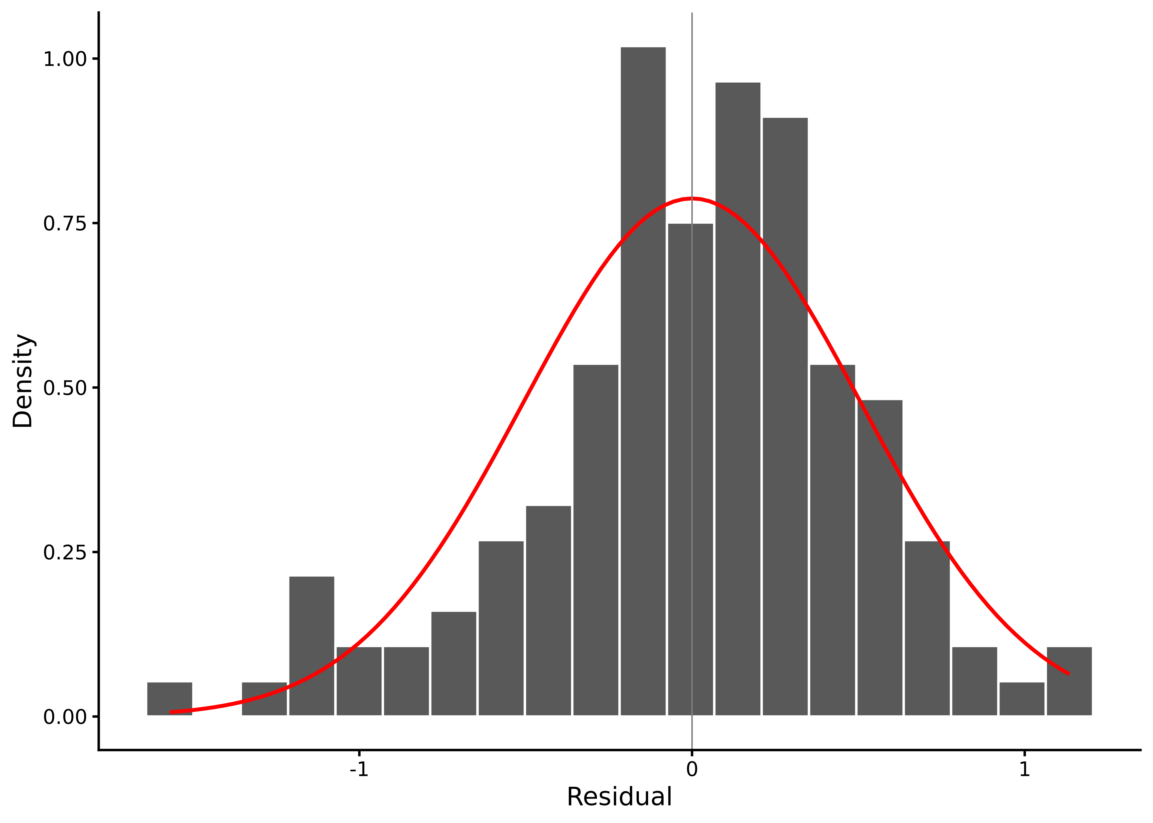
In this histogram, the residuals are centred near zero, roughly symmetrical, with a moderate left skew.
The skewness and kurtosis estimates and their bootstrap intervals provide quantitative information that backs up the histogram.
residual_shape_ci(M_8_1)# A tibble: 2 × 4
measure estimate lower upper
<chr> <dbl> <dbl> <dbl>
1 skewness -0.599 -0.981 -0.180
2 kurtosis 3.68 2.89 4.69 The skew interval lies below zero, confirming a modest negative skew, while kurtosis is close to the normal distribution benchmark of 3.
8.10.2 Residuals versus fitted values
A residuals versus fitted plot shows how the model’s prediction errors vary across the range of predicted values, letting us spot non-linearity, unequal variance, or outlier patterns that would violate regression assumptions (see Section 7.6.2 for more details and Figure 8.4):
lm_diagnostic_plot(M_8_1, type = "resid")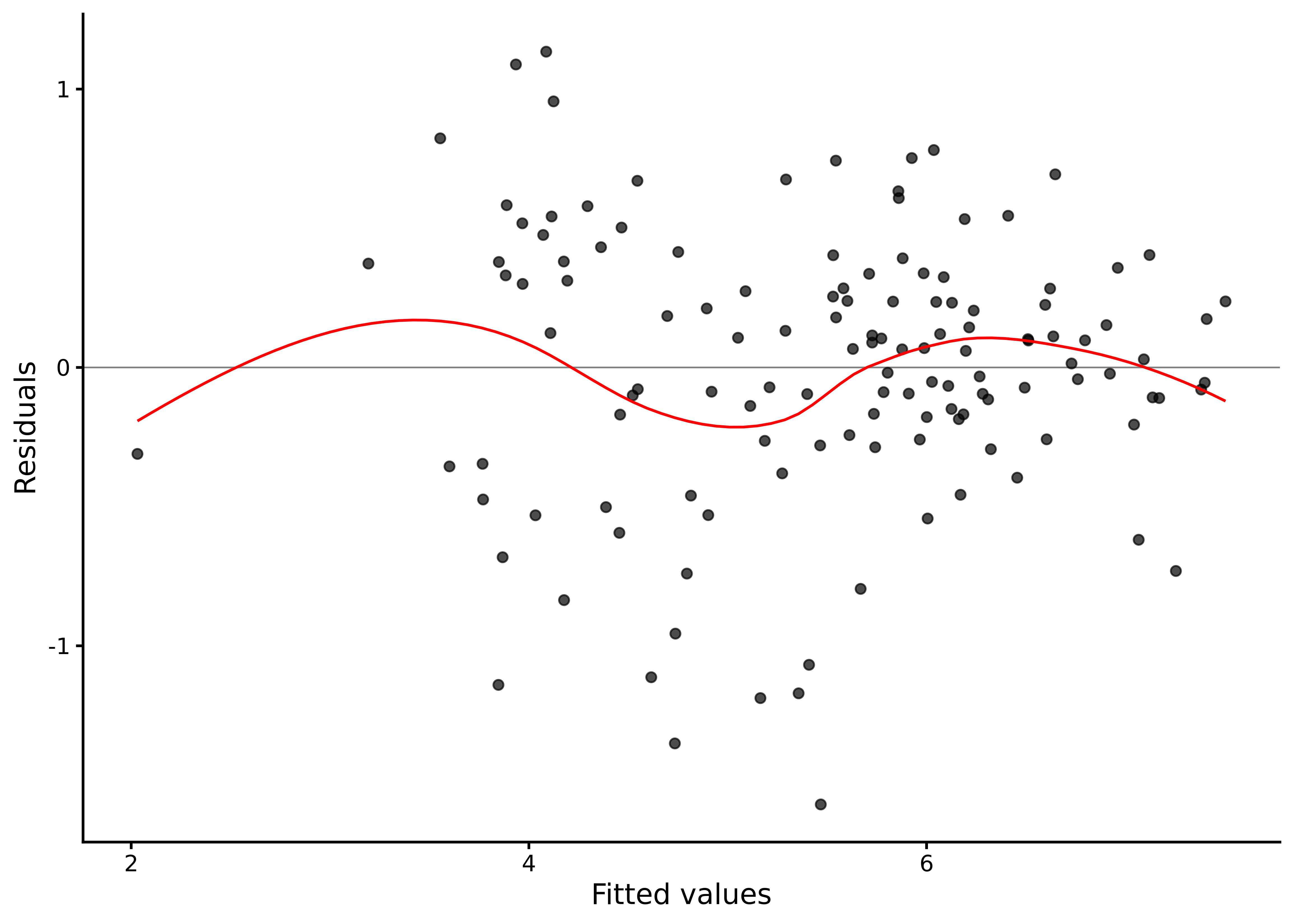
The scatter of residuals forms a roughly horizontal band, with no systematic curve, so a linear mean in all six predictors looks adequate. The spread is fairly even across fitted values, suggesting constant variance. Most points fall within approximately \(\pm 2\hat\sigma\), where \(\hat\sigma = 0.51\).
8.10.3 Normal Q–Q plot
A Q–Q plot compares the ordered residuals with the corresponding quantiles of a normal distribution, revealing whether the residuals follow normality by how closely the points track the diagonal reference line (see Section 7.6.3 for more details and Figure 8.5):
lm_diagnostic_plot(M_8_1, type = "qq")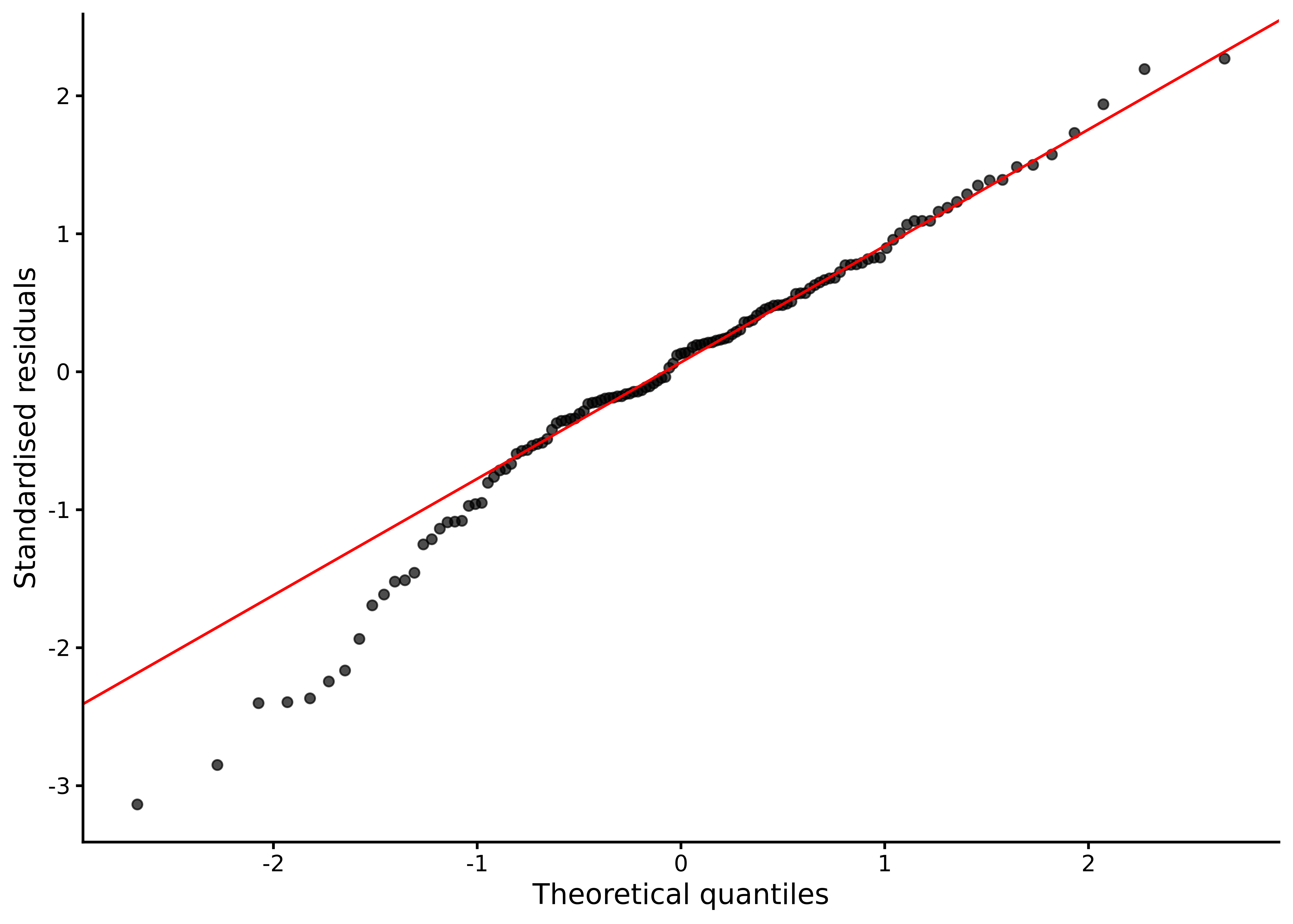
Points follow the reference line closely except for a dip in the lower tail, again in line with the moderate left skew.
Examination of variance homogeneity and leverage statistics using additional diagnostic tools confirms no serious heteroskedasticity and no single influential case dominating the fit.
8.10.4 Diagnostic summary
Across all displays, the multiple-regression model meets its assumptions sufficiently well for most practical purposes. Residuals show moderate left skew, but otherwise the normal-linear model assumptions are met.
As a robustness check, we can compare percentile bootstrap intervals for the coefficients with the usual confidence intervals.
lm_bootstrap_ci(M_8_1)# A tibble: 7 × 4
term estimate lower upper
<chr> <dbl> <dbl> <dbl>
1 (Intercept) -2.29 -3.62 -0.838
2 lgdp 0.328 -0.144 0.872
3 support 3.79 2.46 5.03
4 hle 0.0358 -0.00703 0.0684
5 freedom 2.30 1.37 3.27
6 generosity 0.101 -0.463 0.720
7 corruption -0.915 -1.46 -0.347 confint(M_8_1) 2.5 % 97.5 %
(Intercept) -3.623829943 -0.95933943
lgdp -0.095341898 0.75135095
support 2.576159973 4.99772241
hle 0.007507643 0.06409123
freedom 1.386574804 3.20726377
generosity -0.519752688 0.72190257
corruption -1.528709896 -0.30124688The two sets of intervals are relatively close, although the bootstrap intervals are somewhat wider in some cases. This reinforces the conclusion that the minor deviations from normality have minimal practical effect on our estimates.
8.11 Further reading
Lee Jones et al.’s “Common misconceptions held by health researchers when interpreting linear regression assumptions” (Jones et al., 2025) analyses 95 published studies and reveals that fewer than half reported checking assumptions, highlighting frequent misunderstandings about residual normality, collinearity, and linearity.
Jan Vanhove’s “Collinearity isn’t a disease that needs curing” (Vanhove, 2021) provides a clear discussion of what multicollinearity actually means and why overzealous corrections can distort results or change the research question.
8.12 Chapter summary
- Multiple linear regression extends simple regression by modelling the outcome as a linear function of several predictors simultaneously, with each observation following a normal distribution whose mean depends on all predictors.
- Each regression coefficient represents the expected change in the outcome for a one-unit increase in its corresponding predictor while holding all other predictors constant, capturing partial rather than total associations.
- Coefficients from multiple regression often differ from those in simple regression because multiple regression accounts for overlap among predictors, revealing unique contributions rather than confounded relationships.
- \(R^2\) measures the proportion of variance explained by the model, while adjusted \(R^2\) penalises model complexity and provides a more honest estimate when comparing models with different numbers of predictors.
- F-tests compare nested models to assess whether adding or removing predictors significantly improves fit, with large F-statistics indicating that the additional predictors collectively explain meaningful variation beyond chance.
- Collinearity occurs when predictors are highly correlated with each other, inflating standard errors and destabilising coefficient estimates, detectable using the variance inflation factor (VIF).
- Categorical predictors enter regression as dummy variables, with coefficients representing group differences relative to a chosen reference category, extending regression to handle ANOVA-style designs.
- Interaction terms model how the effect of one predictor changes depending on the value of another, allowing slopes or group differences to vary across levels of a moderating variable.
- Model diagnostics using residual plots, Q-Q plots, and leverage statistics assess assumptions of linearity, homoscedasticity, normality, and identify influential observations that disproportionately affect the fitted model.
- Multiple regression unifies analysis of continuous and categorical predictors under one framework, forming the conceptual foundation for ANOVA, ANCOVA, factorial designs, and the broader general linear model.