14 Bayesian data analysis

In this book, we have covered one approach to inference, namely the classical, also known as frequentist or sampling theory-based, approach. This is the traditional approach to inference. It was by far the dominant approach for most of the twentieth century, and is still the approach that is most widely taught in data analysis courses. However, there is another major approach to statistical inference, which is known as Bayesian inference. While marginalised for most of the twentieth century, towards the end of the 1980s, Bayesian methods began to be used increasingly widely in statistical data analysis, and that usage has continued to grow ever since. Now, Bayesian methods for inference are part of mainstream statistical data analysis. We will introduce them here.

14.1 This chapter covers

The logic of Bayesian inference.
Understand how Bayes’ theorem updates prior beliefs in light of observed data to form the posterior distribution.
Bayesian vs classical perspectives.
Compare the interpretations of probability, uncertainty, and inference under Bayesian and frequentist frameworks.
Priors, likelihoods, and posteriors.
Learn how to specify a prior, calculate a likelihood, and derive a posterior distribution, using simple binomial and normal examples.
Closed-form and simulation-based inference.
See when analytic posteriors can be derived and when sampling methods such as Markov chain Monte Carlo (MCMC) are required.
Markov chain Monte Carlo algorithms.
Explore the logic of Metropolis–Hastings and Hamiltonian Monte Carlo, and how they enable efficient sampling from complex posteriors.
Using Stan and brms for Bayesian modelling.
Fit Bayesian models in R via the brms package, which interfaces with Stan’s high-performance samplers.
Bayesian regression models.
Apply Bayesian approaches to linear, multilevel, logistic (binary, categorical, ordinal), and count models, interpreting posterior estimates and credible intervals.
Model diagnostics and interpretation.
Assess convergence with $\hat{R}$ and effective sample sizes, interpret posterior uncertainty, and compare Bayesian results with their classical counterparts.

Note 14.1: A brief history of Bayesian inference

The origin of Bayesian inference can be traced to a posthumously published 1763 essay titled “Towards Solving a Problem in the Doctrine of Chances,” written some years earlier (Bayes, 1763) by Reverend Thomas Bayes (1701-1761). In this essay, Bayes focused on a problem that is mathematically identical to the problem of inferring the bias of a coin after observing the outcome of a sequence of flips of that coin. Bayes showed that the probability that the coin’s bias is exactly $\theta$ is proportional to the prior probability of $\theta$ multiplied by the probability of the observed outcomes given $\theta$.

Shortly after the publication of Bayes’s essay, the French polymath Pierre-Simon Laplace (1749-1827) independently rediscovered Bayes’ theorem and began to apply it to practical problems of data analysis. Laplace was the first to present Bayesian inference in what is now its modern form: \[ \text{Posterior} = \frac{\text{likelihood} \times \text{prior}}{\text{marginal likelihood}} \] or more formally:

\[ P(\theta | \text{data}) = \frac{P(\text{data} | \theta) P(\theta)}{\int P(\text{data} | \theta) P(\theta) d\theta} \]

By the early 20th century, a frequentist definition of probability became increasingly widely adopted. Crucially, frequentism entails that the concept of probability only applies to the outcomes of random physical processes. As such, a parameter such as the bias of a coin, being a fixed but unknown quantity, cannot be given a probabilistic interpretation. From this perspective, in the words of R. A. Fisher, Bayesian methods were “founded upon an error, and must be wholly rejected” because “inferences respecting populations, from which known samples have been drawn, cannot be expressed in terms of probability” (Fisher, 1925).

Bayesian methods remained marginalised from the early to the late 20th century. However, their potential practical advantage over classical methods was that they could be applied in principle to any problem where a probabilistic model of data could be specified. When computer power was minimal, any “in principle” advantages of Bayesian methods were not important. However, the roughly exponential growth of computational power from the 1970s onwards was the eventual catalyst for the adoption of Bayesian methods. By the late 1980s, Bayesian methods began returning to widespread use in science.

14.2 Bayesian inference

The Bayesian approach to inference calculates the probability distribution over the possible values of the unknown quantities that we are trying to infer, and does this on the basis of the observed values of the data. Returning to our focal example about drug use from Chapter 4, the unknown quantity that we are trying to infer is the proportion of young people who take illegal drugs in Britain. Let us denote this proportion by the symbol $\theta$. By definition, $\theta$ takes values between $0$ and $1$. The Bayesian approach to inference in this case is to calculate the probability that $\theta$ takes any given value, denoted $\tilde{\theta}$, based on the observed data, namely $m=172$ drug users in $n=1300$ survey respondents. Using mathematical notation, we can denote the probability as follows: \[ \mathrm{P}\!\left(\theta = \tilde{\theta} \,\mid\,m = 172, n = 1300\right). \] By calculating this for all possible values of $\tilde{\theta}$ from $0$ to $1$, we obtain a probability distribution over $0$ and $1$ that represents precisely which of the possible values of $\theta$ are or are not probable on the basis of the data that we have observed.

The way we calculate this probability distribution is using a mathematical rule known as Bayes’ theorem or Bayes’ rule. This rule has its origin in a 1763 posthumously published essay by an English Presbyterian minister, The Reverend Thomas Bayes (see Figure 14.1), and so it is named in his honour. Any approach to statistical inference that calculates the probability distribution over the unknown quantities using Bayes’ theorem is known as Bayesian inference.

Figure 14.1: The Reverend Thomas Bayes (1701-1761) was an English Presbyterian minister, who lived and worked in London and then later in Tunbridge Wells in Kent. Bayes was elected a Fellow of the Royal Society, which is a prestigious scientific academy, and the oldest one in continuous existence in the world. After Bayes’s death in 1761, a mathematical essay that he wrote entitled was presented to the Royal Society in Bayes’s name by his friend Richard Price, who was also a Fellow of the Royal Society. This essay contained the result that we now refer to as Bayes’ theorem. The portrait shown here is purportedly that of Bayes, though some doubt that this is the case due to the details of the style of clothing. However, there is no other known portrait of Bayes and this one is used extremely widely.

Bayes’ theorem is a means of inverting conditional probabilities. To understand the meaning of that statement, and how it can be used for statistical inference, let us first describe what conditional probabilities are. A conditional probability is the probability of something happening given that we know something else. Or more precisely, it is the probability that one variable takes a certain value given that another variable takes another value. As an example, consider two binary variables labelled smoker and cancer. The first, smoker, indicates whether a person is a smoker or not. The second, cancer, indicates whether a person ever gets lung cancer in their lifetime or not. The probability that a randomly chosen person is a smoker is denoted by $\mathrm{P}\!\left(\textrm{smoker} = \textrm{yes}\right)$. Likewise, the probability that a randomly chosen person ever gets lung cancer in their lifetime is denoted by $\mathrm{P}\!\left(\textrm{cancer} = \textrm{yes}\right)$. These are unconditional probabilities. They are the probabilities that variables take certain values, but they are not based on knowing the values of other variables. Now consider the probability that a randomly chosen person ever gets lung cancer given that that person is a smoker. This is a conditional probability, and is denoted $\mathrm{P}\!\left(\textrm{cancer} = \textrm{yes} \,\mid\,\textrm{smoker} = \textrm{yes}\right)$. We read the vertical bar, i.e. $|$, as given. This is the probability that a randomly chosen person who smokes ever gets lung cancer in their lifetime. Another conditional probability is $\mathrm{P}\!\left(\textrm{smoker} = \textrm{yes} \,\mid\,\textrm{cancer} = \textrm{yes}\right)$. This is the probability that a person who ever had lung cancer is a smoker.

The two conditional probabilities $\mathrm{P}\!\left(\textrm{cancer} = \textrm{yes} \,\mid\,\textrm{smoker} = \textrm{yes}\right)$ and $\mathrm{P}\!\left(\textrm{smoker} = \textrm{yes} \,\mid\,\textrm{cancer} = \textrm{yes}\right)$ do not mean the same thing and are not identical. If we know one, we do not necessarily know the other. However, Bayes’ theorem allows us to invert conditional probabilities (see Note 14.2 for how Bayes’ theorem works). In other words, it allows us to calculate one conditional probability statement from its inverse. For example, it allows us to calculate $\mathrm{P}\!\left(\textrm{smoker} = \textrm{yes} \,\mid\,\textrm{cancer} = \textrm{yes}\right)$ from $\mathrm{P}\!\left(\textrm{cancer} = \textrm{yes} \,\mid\,\textrm{smoker} = \textrm{yes}\right)$. The calculation for doing so is as follows: \[ \mathrm{P}\!\left(\textrm{smoker} = \textrm{yes} \,\mid\,\textrm{cancer} = \textrm{yes}\right) = \frac{ \mathrm{P}\!\left(\textrm{cancer} = \textrm{yes} \,\mid\,\textrm{smoker} = \textrm{yes}\right) \mathrm{P}\!\left(\textrm{smoker} = \textrm{yes}\right) }{ \mathrm{P}\!\left(\textrm{cancer} = \textrm{yes}\right) } \] The lifetime probability of lung cancer for smokers is around 14%, while for non-smokers it is around 2%, and the approximate proportion of adults who smoke worldwide is around 30%. These values then entail that the overall probability of lung cancer is approximately 6%. Thus, if we know these values, or at least provisionally assume them to be true, then this calculation is as follows: \[ \begin{aligned} \mathrm{P}\!\left(\textrm{smoker} = \textrm{yes} \,\mid\,\textrm{cancer} = \textrm{yes}\right) &= \frac{ 0.14 \times 0.3 }{ 0.06 } = 0.7. \end{aligned} \] In other words, the probability that a person who gets lung cancer is a smoker is 70%.

Note 14.2: Bayes’ theorem

Using some basic rules of probability theory, Bayes’ theorem can be proved with some simple algebra. Let us consider two variables, denoted $X$ and $Y$. The probability that $X$ takes a particular value $x$, and at the same time $Y$ takes a particular value $y$ is denoted $\mathrm{P}\!\left(X = x, Y = y\right)$. Probabilities of combinations of values of multiple variables are known as joint probabilities. A basic rule in probability theory tells us how we can obtain a conditional probability (see main text) from a joint probability. For example, \[ \mathrm{P}\!\left(X = x \,\mid\,Y = y\right) = \frac{\mathrm{P}\!\left(X = x, Y = y\right)}{\mathrm{P}\!\left(Y = y\right)}. \]

The conditional probability $\mathrm{P}\!\left(Y = y \,\mid\,X = x\right)$ can be obtained in the same way: \[ \mathrm{P}\!\left(Y = y \,\mid\,X = x\right) = \frac{\mathrm{P}\!\left(X = x, Y = y\right)}{\mathrm{P}\!\left(X = x\right)}. \] Rearranging this formula we obtain $\mathrm{P}\!\left(X = x, Y = y\right) = \mathrm{P}\!\left(Y = y \,\mid\,X = x\right)\mathrm{P}\!\left(X = x\right)$. If we substitute this into the first equation above, we then obtain Bayes’ rule: \[ \mathrm{P}\!\left(X = x \,\mid\,Y = y\right) = \frac{\mathrm{P}\!\left(Y = y \,\mid\,X = x\right)\mathrm{P}\!\left(X = x\right)}{\mathrm{P}\!\left(Y = y\right)}. \] We can write Bayes’ rule in a more detailed way by using another probability rule: \[ \mathrm{P}\!\left(Y = y\right) = \sum_{\{x\}}\mathrm{P}\!\left(X = x, Y = y\right). \] This tells us that if we sum over all values of $X$ (the $\{x\}$ in the limits of the sum denotes the set of all possible values of $X$) in the joint probability of $X$ and $Y$, we obtain the probability of $Y$ alone. Writing the joint probability $\mathrm{P}\!\left(X = x, Y = y\right)$ as $\mathrm{P}\!\left(Y = y \,\mid\,X = x\right)\mathrm{P}\!\left(X = x\right)$, we then can replace the denominator in the Bayes’ rule equation above by the following: \[ \mathrm{P}\!\left(X = x \,\mid\,Y = y\right) = \frac{\mathrm{P}\!\left(Y = y \,\mid\,X = x\right)\mathrm{P}\!\left(X = x\right)}{\sum_{\{x\}}\mathrm{P}\!\left(Y = y \,\mid\,X = x\right)\mathrm{P}\!\left(X = x\right) }. \] This form is usually the preferred form of Bayes’ rule as it shows how the denominator is calculated. Note that if the $X$ variable here is continuous, the sum in the denominator would be replaced by an integral, i.e. $\int \mathrm{P}\!\left(Y = y \,\mid\,X = x\right)\mathrm{P}\!\left(X = x\right) dx$.

Let us now turn to how we can use Bayes’ theorem for statistical inference. For the drug use problem, with Bayesian statistical inference, we aim to calculate the probability, based on the observed data of $m=172$ drug users in $n=1300$ survey respondents, that this unknown proportion $\theta$ takes any value, denoted by $\tilde{\theta}$, between $0$ and $1$. We write this probability as $\mathrm{P}\!\left(\theta = \tilde{\theta} \,\mid\,m = 172, n = 1300\right)$. Note that we must calculate this for all possible values of $\tilde{\theta}$ from $0$ to $1$. This gives us a function over the interval from $0$ to $1$. For every value of $\tilde{\theta}$ in the interval from $0$ to $1$, this function gives us the probability that $\theta$ takes that value. This probability function is known as the posterior distribution, and so $\mathrm{P}\!\left(\theta = \tilde{\theta} \,\mid\,m = 172, n = 1300\right)$ is said to be the posterior probability that the population variable $\theta$ takes the value of $\tilde{\theta}$.

We calculate the posterior probability that $\theta = \tilde{\theta}$ with Bayes’ theorem as follows: \[\begin{equation} \mathrm{P}\!\left(\theta = \tilde{\theta} \,\mid\,m = 172, n = 1300\right) = \frac{\mathrm{P}\!\left(m = 172 \,\mid\,\theta = \tilde{\theta}, n = 1300\right) \mathrm{P}\!\left(\theta = \tilde{\theta}\right)}{\mathrm{P}\!\left(m = 172 \,\mid\,n = 1300\right)}. \end{equation}\]

There are three terms on the right-hand side of this equation. The first term in the numerator is $\mathrm{P}\!\left(m = 172 \,\mid\,\theta = \tilde{\theta}, n = 1300\right)$. This gives the probability of observing $m=172$ drug users in a sample of $n=1300$, assuming the true proportion of drug users in the population is exactly $\theta = \tilde{\theta}$. We calculate this quantity for all values of $\tilde{\theta}$ from $0$ to $1$. This gives us, as was the case for the posterior distribution, a function over the interval from $0$ to $1$. For every value of $\tilde{\theta}$ in the interval from $0$ to $1$, this function gives us the probability of observing $m=172$ drug users in a sample of $n=1300$ assuming the population proportion $\theta$ takes the value of $\tilde{\theta}$. This function is known as the likelihood function, which is a particularly important function in statistics generally, both in the Bayesian and classical approaches. It is shown in Figure 14.2(a). The likelihood function at $\theta = \tilde{\theta}$ gives the evidence in favour of $\theta$ having the value of $\tilde{\theta}$. As we can see, the data provide nontrivial evidence in favour of values from around 0.11 to around 0.16. Values of $\theta$ outside this interval have a very low degree of evidence in their favour. We also see that this function takes its maximum around $\theta = 0.13$. In other words, the data provide most evidence in favour of $\theta = 0.13$, but it can be shown that any value of $\theta$ in the interval from around $0.11$ to around $0.16$ has evidence that is at least a certain fraction, specifically $\frac{1}{32}$, of the maximum evidence at $\theta = 0.13$.

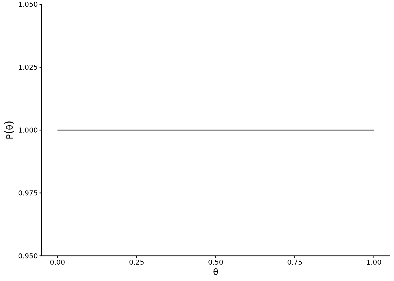
Figure 14.2: a) The likelihood function for the drug user proportion problem. The likelihood function tells us how much evidence is provided by the data for each possible value of the population proportion, signified by $\theta$. Clearly, the data provide negligible evidence for values below around 0.1 and above around 0.16. b) A uniform prior over the population proportion $\theta$. A uniform prior represents our assumption that all values of $\theta$ are in principle equally probable before we have observed any data.

The second term in the numerator of the Bayes rule equation is $\mathrm{P}\!\left(\theta = \tilde{\theta}\right)$. This is known as the prior probability, or simply the prior. The prior allows us to specify the range of possible values that $\theta$ can take, and what their relative probabilities are. Ultimately, the prior is an assumption, but one that should, like any assumption in statistical analysis, be reasonable and based on what is known about the problem at hand. In Section 6.4, we discussed the general topic of assumptions in statistical models, and these discussions will allow us to further discuss what priors are and how to choose them. For now, we will keep matters very simple and just assume that $\theta$ could have any possible value with equal probability. This is known as a uniform prior. It is a flat line function over $\theta$, see Figure 14.2(b).

Figure 14.3: The posterior distribution for the possible values of the population proportion of drug users, signified by $\theta$, based on the observed data. This distribution tells us which values of $\theta$ are and are probable according to the data. Clearly, we see that only values from around 0.1 to 0.16 have any nontrivial degree of probability. Shown in red is the 95% high posterior density interval. There is a 95% probability that the true value of $\theta$ is in that interval.

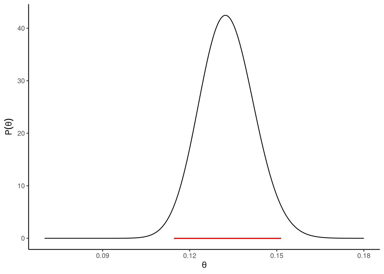
Now that we have our likelihood function and our prior, we know how to evaluate both terms in the numerator of the Bayes rule equation. We then multiply these terms by one another. In other words, for any value of $\tilde{\theta}$, we multiply $\mathrm{P}\!\left(m = 172 \,\mid\,\theta = \tilde{\theta}, n = 1300\right)$ by $\mathrm{P}\!\left(\theta = \tilde{\theta}\right)$. We then divide this value by the denominator of the equation, i.e. $\mathrm{P}\!\left(m = 172 \,\mid\,n = 1300\right)$. It turns out (see Note 14.2) that we can calculate this using an integral over the product of $\mathrm{P}\!\left(m = 172 \,\mid\,\theta = \tilde{\theta}, n = 1300\right)$ and $\mathrm{P}\!\left(\theta = \tilde{\theta}\right)$. This integral is known as the marginal likelihood. As such, to obtain the posterior distribution, for all possible values of $\tilde{\theta}$, we multiply $\mathrm{P}\!\left(m = 172 \,\mid\,\theta = \tilde{\theta}, n = 1300\right)$ by $\mathrm{P}\!\left(\theta = \tilde{\theta}\right)$ and then divide by the marginal likelihood. This posterior is shown in Figure 14.3. One useful way to think about the posterior distribution is that it is obtained by first multiplying two functions, the likelihood and the prior, by one another to produce a new function. This new product function is what is given by the numerator of the Bayes rule equation. We then calculate the area under the curve of this new function. That is the marginal likelihood, which we said is calculated using an integral, and an integral gives the area under a function. We then divide the product function by the marginal likelihood to produce the posterior distribution. This dividing of the product function by the marginal likelihood is also known as normalising the function. It guarantees that the resulting posterior distribution is a true probability distribution, with the area under the posterior distribution being always exactly 1.0.

The posterior distribution shown in Figure 14.3 tells us everything we know about the true value of the population proportion $\theta$ based on the data that we have observed and the various assumptions that we have made. We can provide a rough summary of this distribution in terms of its mean and standard deviation. For a problem like the current one, we can obtain these from the binomial_posterior_summary function in sgsur:

binomial_posterior_summary(sample_size = 1300, observed = 172)

       mean          sd 
0.132872504 0.009403442

We can therefore summarise what we know about $\theta$ by saying it has a distribution of possible values whose mean is 0.133 and whose standard deviation is 0.009. The posterior mean is essentially our best estimate of $\theta$, while the posterior standard deviation tells us how much uncertainty we have about this estimate. The greater the value of the standard deviation, the more uncertainty we have. As a rough rule of thumb, which we will also often see elsewhere, we can multiply the standard deviation of 0.009 by 2.0, and add and subtract that to or from the mean of 0.133. That gives us the range from 0.114 to 0.152. This is, roughly speaking, the range of possible values of $\theta$ that have a relatively high probability. In other words, roughly speaking, on the basis of having obtained 172 drug users in 1300, we can say that there is a high probability that the true proportion of drug users in the population, $\theta$, is between 0.114 and 0.152.

We can be even more precise in our summary of the posterior distribution. For example, we can show that the probability that the true value of $\theta$ is between 0.115 and 0.151 is exactly 95%. This interval, which is known as the 95% high posterior density (HPD) interval, is shown as the red line in Figure 14.3. Any value of $\theta$ in that interval has a higher probability than any value outside of it, and the total probability of a value of $\theta$ being in that interval is exactly 95%. This HPD interval is comparable to the confidence interval we discussed in the previous section in the sense that it gives us a range of values of $\theta$ that have a degree of support from the data in some sense. However, the meanings and the interpretations of the classical confidence interval and the HPD interval are different. The classical 95% confidence interval is the range of values of $\theta$ that have a hypothesis test p-value of $p > 0.05$. In other words, these are the range of values of $\theta$ that are compatible with the data according to hypothesis tests. As mentioned earlier, a common misinterpretation of the 95% confidence interval is that there is a 95% probability that the true value of $\theta$ is in the range. On the other hand, this is the correct interpretation of the 95% HPD interval. It is true that the probability that $\theta$ is in the 95% HPD interval is exactly 95%. In other words, in this case, we can be 95% certain that the true value of $\theta$ is between 0.115 and 0.151.

From the sgsur package, we can calculate the interval for the current problem as follows:

binomial_posterior_hpd(sample_size = 1300, observed = 172)

    0.025     0.975 
0.1146233 0.1514224

This, by default, uses a uniform prior, which is the one we are using now, but that can be changed. By default, it also returns the 95% interval. To obtain, for example, the 99% interval, we use level = 0.99 in the function call:

binomial_posterior_hpd(sample_size = 1300, observed = 172, level = 0.99)

    0.005     0.995 
0.1093713 0.1577197

From this, we can see that there is a 99% probability that $\theta$ has a value between around 0.109 and 0.158. We can compare these HPD intervals to their corresponding confidence intervals.

binomial_confint(sample_size = 1300, observed = 172)

    0.025     0.975 
0.1143520 0.1519436

binomial_confint(sample_size = 1300, observed = 172, level = 0.99)

    0.005     0.995 
0.1091052 0.1582544

Clearly, the confidence intervals and the HPD intervals are very similar in this case. In many common problems, the classical confidence intervals and the Bayesian HPD intervals are similar. Sometimes, in fact, they are identical. Nonetheless, it is important to remember that they mean different things, and are interpreted differently, and may not necessarily have similar values.

14.3 Bayesian inference in normal distributions

Let us now consider Bayesian inference of the mean $\mu$ of a normal distribution. Our starting point is identical to that of the classical approach. Specifically, we assume we have $n$ independent observations that can be represented as follows \[ y_1, y_2, \ldots y_n, \] and we assume the following model: \[ y_i \sim N(\mu, \sigma^2),\quad\text{for $i \in 1 \ldots n$}, \] where both $\mu$ and $\sigma$ have fixed but unknown values. Inference in Bayesian approaches, just like in classical approaches, aims to infer what these values are. As we mentioned above, the theoretical basis of Bayesian inference differs markedly from the classical approach. Nonetheless, and just as we saw earlier, the ultimate conclusions may still be remarkably similar to one another.

The fundamental point of departure between the classical and the Bayesian approaches is that the Bayesian approach assumes that the unknown variables in the model, which are $\mu$ and $\sigma$ in this case, have been drawn from some prior distribution. We can therefore write our statistical model as follows: \[ \begin{aligned} y_i &\sim N(\mu, \sigma^2),\quad\text{for $i \in 1 \ldots n$},\\ \mu, \sigma &\sim \mathrm{P}\!\left(\mu, \sigma\right) \end{aligned} \] where $\mathrm{P}\!\left(\mu, \sigma\right)$ just indicates some as yet unspecified probability distributions over $\mu$ and $\sigma$. Having specified the prior, we can now use Bayes’ theorem to calculate the posterior probability distribution over $\mu$ and $\sigma$. Writing $\vec{y}$ for $y_1, y_2 \ldots y_n$, the posterior distribution can be written as follows. \[ \overbrace{\mathrm{P}\!\left(\mu, \sigma \,\mid\,\vec{y}\right)}^{\textrm{posterior}} = \frac{ \overbrace{\mathrm{P}\!\left(\vec{y} \,\mid\,\mu, \sigma\right)}^{\textrm{likelihood}} \overbrace{\mathrm{P}\!\left(\mu,\sigma\right)}^{\textrm{prior}} }{ \underbrace{\int \mathrm{P}\!\left(\vec{y} \,\mid\,\mu, \sigma\right) \mathrm{P}\!\left(\mu,\sigma\right) d\mu d\sigma}_{\textrm{marginal likelihood}}. } \]

In general across all Bayesian models, the posterior distribution is itself a probability distribution. This means it is a non-negative function that assigns probabilities to all possible values of a parameter and integrates to exactly 1.0 over its range. In other words, it tells us how plausible each possible value of a parameter is, given the data and the model’s assumptions.

Sometimes, we can write this posterior distribution in an explicit mathematical form — called a closed-form or analytic expression. In those cases, we have a formula that can be evaluated directly for any parameter value using straightforward calculations, perhaps even by hand.

However, most Bayesian models are not this simple. The mathematics of combining complex likelihoods and priors usually produces a posterior that cannot be expressed neatly, because the required integrals have no exact solution. When that happens, we must approximate the posterior using computational methods such as Markov chain Monte Carlo (MCMC), as discussed in section 14.3.

For this particular example — Bayesian inference for the mean of a normal distribution — things are simpler. By choosing certain forms of priors that are mathematically compatible with the likelihood (known as conjugate priors), we can obtain a closed-form expression for the posterior distribution. This makes it possible to see exactly how the data and the prior combine to produce our updated beliefs about the mean.

14.3.1 Closed form solution

The first term in the numerator on the right-hand side of Bayes’ rule above is the likelihood function. The likelihood function is not a probability distribution, but is a function over the $\mu$ and $\sigma$ space. It can be written as follows. \[ \begin{aligned} \mathrm{P}\!\left(\vec{y}\,\mid\,\mu, \sigma\right) &= \prod_{i=1}^n \mathrm{P}\!\left(y_i \,\mid\,\mu, \sigma\right),\\ &= \left(\frac{1}{\sqrt{2\pi}}\right)^n \sigma^{-n} \exp\left[- \frac{1}{2\sigma^2} (\vec{y} - \mu)\strut^\intercal (\vec{y} - \mu)\right],\\ &= \left(\frac{1}{\sqrt{2\pi}}\right)^n \sigma^{-n} \exp\left[- \frac{1}{2\sigma^2} \left[(n-1)s^2 + n(\mu-\bar{y})^2\right]\right],\\ \end{aligned} \] where $\bar{y}$ and $s^2$ have identical values to those defined above, namely \[ \bar{y} = \frac{1}{n}\sum_{i=1}^{n} y_i,\quad s^2 = \frac{1}{n - 1} \sum_{i=1}^n | y_i - \bar{y}|^2. \]

The second term in the numerator is the prior. It is a function over the $\mu$ and $\sigma$ space, but of course it is also a probability distribution. In principle, this probability distribution can be from any parametric family that is defined on the $\mu$ and $\sigma$ space. However, as mentioned, in order to obtain an analytic expression for the posterior, we must restrict our choices of probability distributions. One common choice for normal linear models is to use an uninformative prior, specifically one that is uniform over $\mu$ and $\log(\sigma)$. This turns out to be equivalent to \[ \mathrm{P}\!\left(\mu, \sigma\right) \propto \frac{1}{\sigma^2}. \]

The posterior $\mathrm{P}\!\left(\mu, \sigma \,\mid\,\vec{y}\right)$ is the product of the likelihood and the prior, divided by their integral. The resulting distribution is a normal-inverse-Gamma distribution, which can be written in the following factored form. \[ \begin{aligned} \mathrm{P}\!\left(\mu, \sigma \,\mid\,\vec{y}\right) &= \mathrm{P}\!\left(\mu \,\mid\,\sigma, \vec{y}\right) \mathrm{P}\!\left(\sigma \,\mid\,\vec{y}\right),\\ &= N(\mu \,\mid\,\bar{y}, \sigma^2/n)\times\textrm{invGamma}(\sigma^2 \,\mid\,\tfrac{n-1}{2},\tfrac{(n-1)s^2}{2}). \end{aligned} \]

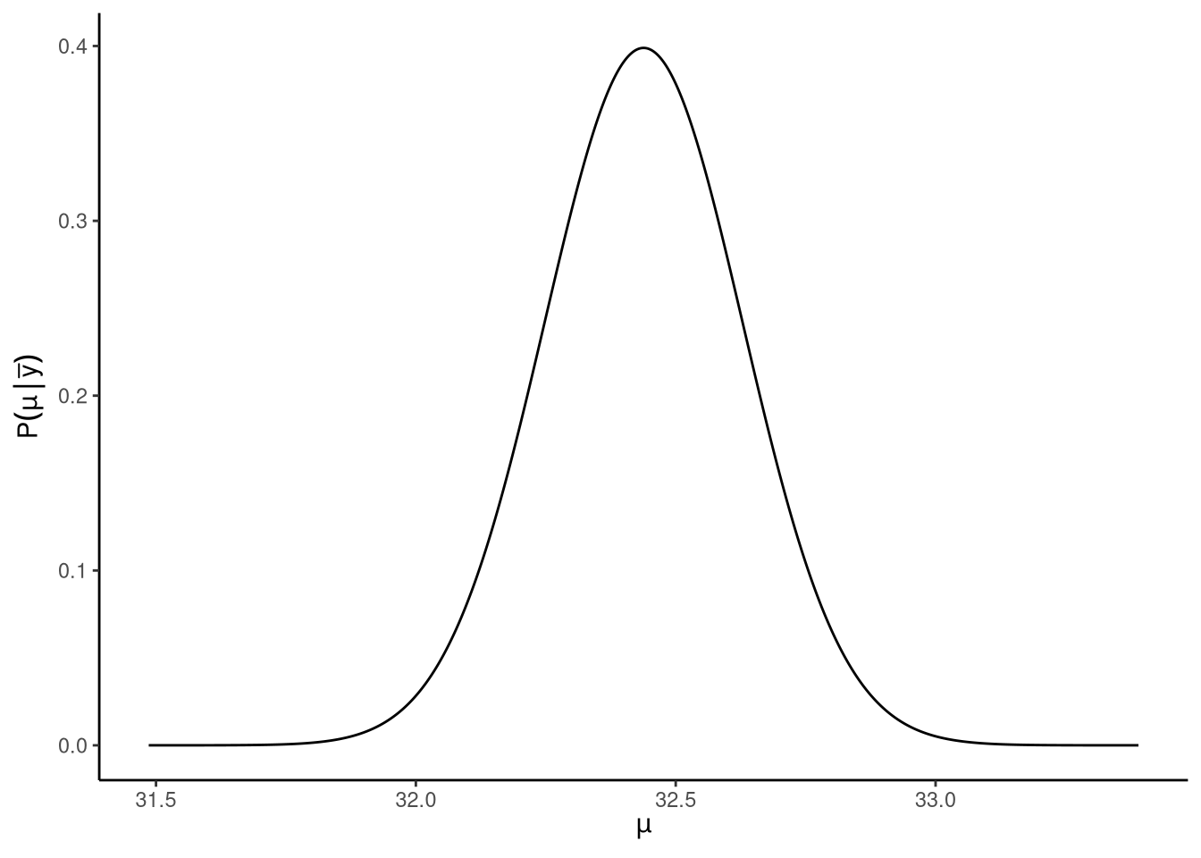
An interesting consequence of this distribution is when we marginalise over the $\sigma^2$, this leads to a non-standard with location parameter $\bar{y}$, scale parameter $s/\sqrt{n}$, and degrees of freedom $n -1$: \[ \mathrm{P}\!\left(\mu\,\mid\,\vec{y}\right) \sim \textrm{t}_{n-1}(\mu\,\mid\,\bar{y}, s^2/n). \] This posterior distribution is shown in Figure 14.4. This entails that the probability, according to the posterior distribution, that the true value of $\mu$ is in the range \[ \bar{y} \pm T(\gamma, n -1) \frac{s}{\sqrt{n}}, \] is $\gamma$. Here, $T(\gamma, \nu)$ was defined above. This gives us the high posterior density () interval for $\mu$. Setting $\gamma = 0.95$, for example, gives us the 95% interval. In other words, according to the posterior distribution, there is a 95% probability that $\mu$ is in the range $\bar{y} \pm T(\gamma, \nu) \frac{s}{\sqrt{n}}$. What is particularly interesting about this result is that it is identical to the 95% confidence interval for $\mu$ defined above.

Figure 14.4: The posterior distribution over $\mu$ given the observed data. This distribution is a non-standard $t$-distribution whose location parameter is $\bar{y}$ and whose scale parameter is $s/\sqrt{n}$.

14.4 Introducing Markov Chain Monte Carlo

In general, given observed data $D$ and a model $\Omega$, the posterior distribution over the parameters $\theta$ of the model is given by: \[ P(\theta | D, \Omega) = \frac{P(D | \theta) P(\theta | \Omega)}{\int P(D | \theta) P(\theta | \Omega) d\theta}. \]

The numerator contains the likelihood $P(D | \theta)$ and the prior $P(\theta | \Omega)$, while the denominator represents the marginal likelihood, which gives the likelihood of the model given the observed data. Given this posterior distribution, our aim is often to characterise this distribution in terms of its mean, variance, and other summary statistics.

A major issue is that in only rare situations can we determine the characteristics of the posterior distribution, or calculate posterior predictive distributions, in closed form. However, if we can draw samples from $P(\theta | D, \Omega)$, then we can calculate anything we need to know about the posterior distribution. For example, we can approximate the mean of the distribution by $\langle\theta\rangle = \int \theta P(\theta | D, \Omega) d\theta \approx \frac{1}{N} \sum_{i=1}^N \tilde{\theta}_i$, the variance by $\text{Var}(\theta) \approx \frac{1}{N} \sum_{i=1}^N (\tilde{\theta}_i - \bar{\theta})^2$, quantiles, credible intervals, or any other summary statistic of interest, where $\tilde{\theta}_1, \tilde{\theta}_2, \ldots, \tilde{\theta}_N$ are samples from $P(\theta | D, \Omega)$. In essence, sampling from the posterior distribution provides a complete solution to Bayesian inference.

The Metropolis-Hastings algorithm provides a practical method for sampling from posterior distributions. Let us denote $P(\theta | D, \Omega)$ by $f(\theta)$. The algorithm works by sampling from a symmetric proposal distribution $Q(\cdot | \cdot)$. Starting with an initial value $\tilde{\theta}_0$, we sample $\tilde{\theta} \sim Q(\theta | \tilde{\theta}_0)$. We then accept $\tilde{\theta}$ with probability $\alpha = \min\left(1.0, \frac{f(\tilde{\theta})}{f(\tilde{\theta}_0)}\right)$. After convergence, the accepted samples are draws from the distribution $f(\theta)$. A key advantage of the Metropolis-Hastings algorithm is that the distribution $f(\theta)$ need only be known up to a proportional constant, which means we can work directly with the unnormalised posterior without computing the often intractable marginal likelihood.

The Metropolis algorithm we have described is known as a random walk Metropolis because it takes random steps in parameter space through its proposal distribution. While effective, this random walk approach suffers from inefficiency, particularly in high-dimensional problems where most random proposals will be to regions of low probability density and will therefore be rejected. Hamiltonian Monte Carlo (HMC) addresses this limitation by using the gradient of the posterior distribution to guide its proposals towards regions of higher probability. Rather than taking random steps, HMC treats the parameters as the position of a particle moving through a physical landscape where the posterior distribution determines the potential energy. The algorithm gives the particle momentum and allows it to move according to the laws of physics, with the gradient of the posterior acting like a force that guides the particle along paths of relatively high probability density. This results in proposals that are much more likely to be accepted and allows the sampler to explore the posterior distribution far more efficiently than random walk methods.

While methods such as HMC give us the ability to sample efficiently from complex posterior distributions, implementing these algorithms from scratch is a substantial undertaking. They require careful coding, numerical stability considerations, and fine-tuning to ensure convergence and efficiency—tasks that are not only time-consuming but also easy to get wrong. Rather than writing our own sampler, we can use well-tested, high-performance software that implements these algorithms for us. This is where Stan comes in.

Stan is an open-source probabilistic programming language designed specifically for statistical modelling and high-performance Bayesian inference. It implements state-of-the-art sampling algorithms, most notably an adaptive form of HMC. Using Stan directly involves writing a model in Stan’s own modelling language, specifying the data, parameters, priors, and likelihood. Stan then compiles this model to C++ code for speed and runs the sampling algorithm to produce posterior draws. The output includes not only samples from the posterior distribution but also diagnostics (such as $\hat{R}$ and effective sample size) to assess convergence and sampling efficiency. While powerful and flexible, writing raw Stan code can be time-consuming, especially for standard models like linear regression, logistic regression, or ANOVA, which have well-known forms.

The brms package in R provides a high-level interface to Stan that allows users to specify Bayesian regression models using R’s familiar model formula syntax. Instead of writing Stan code directly, you write formulas such as:

brm(y ~ x1 + x2, data = df)

and brms generates the corresponding Stan programme behind the scenes. It then compiles and runs the model in Stan, returning posterior samples as standard R objects that integrate seamlessly with other R tools.

brms supports an extremely wide range of models — linear, generalised linear, multilevel, survival, zero-inflated, and many more — while allowing full control over priors and advanced options. The main advantage, and the key point for our purposes, is that brms makes it possible to perform sophisticated Bayesian analyses with almost no more effort than fitting the corresponding frequentist models in lm() or glm(). As we will see in the next section, in many cases you can take your existing regression code, change lm() to brm(), specify priors if you wish, and immediately obtain a full Bayesian analysis powered by Stan.

14.5 Bayesian regression models

To run the following models, we need to load the brms package:

14.5.1 Multiple linear regression

This was one of the lm() models that we ran in Section 8.5:

M_8_1 <- lm(happiness ~ lgdp + support + hle + freedom + generosity + corruption,
            data = whr2024)

We can perform the Bayesian counterpart of this, using default priors, as easily as by changing lm() to brm() and nothing more:

M_8_1_bayes <- brm(
  happiness ~ lgdp + support + hle + freedom + generosity + corruption,
  data = whr2024
)

We can inspect the main results with summary() or just by typing the model’s name:

summary(M_8_1_bayes)

 Family: gaussian 
  Links: mu = identity 
Formula: happiness ~ lgdp + support + hle + freedom + generosity + corruption 
   Data: whr2024 (Number of observations: 131) 
  Draws: 4 chains, each with iter = 2000; warmup = 1000; thin = 1;
         total post-warmup draws = 4000

Regression Coefficients:
           Estimate Est.Error l-95% CI u-95% CI Rhat Bulk_ESS Tail_ESS
Intercept     -2.30      0.69    -3.64    -0.95 1.00     4369     3278
lgdp           0.33      0.22    -0.10     0.75 1.00     3002     2583
support        3.79      0.61     2.58     5.02 1.00     3707     2868
hle            0.04      0.01     0.01     0.06 1.00     3881     3167
freedom        2.30      0.47     1.36     3.20 1.00     4183     2689
generosity     0.10      0.32    -0.53     0.70 1.00     5063     2858
corruption    -0.91      0.32    -1.53    -0.30 1.00     3740     2871

Further Distributional Parameters:
      Estimate Est.Error l-95% CI u-95% CI Rhat Bulk_ESS Tail_ESS
sigma     0.51      0.03     0.45     0.58 1.00     5001     2557

Draws were sampled using sampling(NUTS). For each parameter, Bulk_ESS
and Tail_ESS are effective sample size measures, and Rhat is the potential
scale reduction factor on split chains (at convergence, Rhat = 1).

There is a lot of output here. Some of it will look very familiar, and in fact, there are parallels between classical and Bayesian results, as we explain below. However, technically speaking, everything here is different to what we obtain from the lm() model and some details have no parallels with classical results.

The first block identifies the statistical model that was fit.

Family tells you the probability distribution used for the outcome variable, and here gaussian just means a normal distribution.
Links lists the link function applied to each modelled parameter and here mu, the mean of the normal distribution, uses the identity link, as does sigma, which means both parameters are on their natural scales without transformations.
Formula repeats the R formula you supplied and this confirms which predictors and interactions were included on the right-hand side and which outcome was on the left.
Data reports which data frame was used and how many rows were actually included after any internal handling of missing values.
Draws reports how many Markov chains were run, how many total iterations per chain, how many were used for warmup and adaptation, whether thinning was applied, and how many post-warmup samples remain in total across chains for inference.

The next block is the table of population level regression coefficients. Each row corresponds to one parameter in the linear predictor which includes the intercept and one row for each predictor and factor level coding implied by your formula.

Estimate is the posterior mean of that parameter which is the simple average of its sampled values across all post-warmup draws.
Est.Error is the posterior standard deviation of that parameter which quantifies the dispersion of its sampled values and serves as the Bayesian analogue of a standard error.
l-95% CI and u-95% CI are the lower and upper endpoints of an equal-tailed 95 percent posterior interval, also known as the credible interval, computed from the 2.5th and 97.5th percentiles of the posterior draws. These credible intervals are probability statements about the parameter given the model and the data. You can read them as there is 95 percent posterior probability that the parameter lies between the reported limits.
Rhat is a MCMC convergence diagnostic. Values very close to 1 indicate that the separate chains are mixing well and giving consistent draws while values above about 1.01 suggest lack of convergence that needs investigation.
Bulk_ESS is an effective sample size measure for the bulk of the posterior and it estimates how many independent draws your correlated Markov chain is roughly equivalent to in the central region of the distribution.
Tail_ESS is an analogous effective sample size focused on the tails of the posterior and low values can indicate that extreme quantiles are estimated imprecisely.

It is helpful to read one row in detail to fix ideas. Consider the row for freedom:

The Estimate 2.3 is the posterior mean of the regression coefficient for freedom, which is the average effect size across the 4000 post-warmup draws under this model and coding. If freedom increases by one unit, holding the other predictors fixed at their current values in the model, then the expected happiness increases by about 2.31 units on the outcome scale according to the posterior mean.
Est.Error of 0.47 is the posterior standard deviation for this coefficient, and it summarises the uncertainty in that effect after combining the likelihood with the prior.
The posterior interval from 1.36 to 3.2 is the central 95 percent credible interval which states that given the model and priors and data there is 95 percent probability that the regression coefficient for freedom lies between 1.36 and 3.2.
Rhat equal to 1 indicates excellent between-chain agreement for this parameter which supports the conclusion that the chains have converged for this effect.
Bulk_ESS of 4183 means that the correlated Markov chain draws for the central region of this parameter carry information roughly comparable to about 4183 independent samples.
Tail_ESS of 2689 means the information in the tails of the posterior for this parameter is roughly comparable to about 2689 independent samples, which is usually adequate for estimating tail quantiles and credible intervals.

You can interpret the other predictor rows in the same way.

The block titled Further Distributional Parameters reports parameters beyond the mean structure that belong to the likelihood. For the gaussian family, the additional parameter is sigma, which is the residual standard deviation. The row for sigma is summarised exactly like the coefficients with a posterior mean, a posterior standard deviation, a 95 percent credible interval, and the same convergence and efficiency diagnostics. A smaller sigma indicates tighter residual scatter around the regression line, while a larger sigma indicates more residual variability not explained by the predictors.

The final lines summarise how sampling was performed. Draws were obtained using the NUTS algorithm, which is an adaptive form of Hamiltonian Monte Carlo that uses gradients of the log posterior to make long-distance proposals with high acceptance probabilities. The reminder that Bulk_ESS and Tail_ESS are effective sample size measures and that Rhat is the potential scale reduction factor emphasises that these diagnostics should be checked to ensure reliable inference before interpreting estimates and intervals.

There are two additional points that are not printed but are important for interpretation. Unless you set priors explicitly, brms uses its default priors for the family and parameters, and you can inspect exactly what was used with prior_summary() on the fitted model object. If you want posterior probabilities for directional claims such as the probability that a coefficient is greater than zero, or region of practical equivalence summaries, you can compute them directly from the stored posterior draws that brms keeps in the fit object.

14.5.2 Multilevel linear models

Running a Bayesian equivalent of the multilevel model is straightforward using brms. We’ll run just the random intercepts and random slopes model used in Section 11.5, but the syntax can easily be amended to change the specification of the model.

sleep_bayes <- brm(Reaction ~ Days + (Days|Subject), data = sleepstudy)

Results of the model can be accessed using summary(sleep_bayes)

summary(sleep_bayes)

 Family: gaussian 
  Links: mu = identity 
Formula: Reaction ~ Days + (Days | Subject) 
   Data: sleepstudy (Number of observations: 180) 
  Draws: 4 chains, each with iter = 2000; warmup = 1000; thin = 1;
         total post-warmup draws = 4000

Multilevel Hyperparameters:
~Subject (Number of levels: 18) 
                    Estimate Est.Error l-95% CI u-95% CI Rhat Bulk_ESS Tail_ESS
sd(Intercept)          26.91      6.67    15.85    42.00 1.00     1715     2571
sd(Days)                6.61      1.53     4.23    10.12 1.00     1354     1980
cor(Intercept,Days)     0.08      0.30    -0.48     0.66 1.00     1034     1754

Regression Coefficients:
          Estimate Est.Error l-95% CI u-95% CI Rhat Bulk_ESS Tail_ESS
Intercept   250.91      7.24   236.51   265.54 1.00     1997     2328
Days         10.48      1.68     7.05    13.70 1.00     1650     1938

Further Distributional Parameters:
      Estimate Est.Error l-95% CI u-95% CI Rhat Bulk_ESS Tail_ESS
sigma    25.90      1.52    23.12    29.12 1.00     3735     2683

Draws were sampled using sampling(NUTS). For each parameter, Bulk_ESS
and Tail_ESS are effective sample size measures, and Rhat is the potential
scale reduction factor on split chains (at convergence, Rhat = 1).

Similar to the classical inference model, we see the output split into sections. The group level effects refer to our ‘random effects’, and are here accompanied by standard errors and a 95% credible interval. The population level effects provide the population intercept and slope, whilst the family specific parameters provide the estimate of sigma.

14.5.3 Binary logistic regression

Modelling the data using Bayesian inference begins with the same model that we specified in Chapter 12, that is: \[ \begin{aligned} y_i &\sim \textrm{Bernoulli}(\theta_i),\quad\text{for $i \in 1, 2 \ldots n$},\\ \ln\left(\frac{\theta}{1 - \theta}\right) &= \beta_0 + \sum_{k=1}^K \beta_k x_{ki}. \end{aligned} \]

We can specify this model using brm(), in a very similar way to what we did in Chapter 12 with glm():

volunteer_m_bayes <- brm(volunteer ~ extraversion,
                         data = volunteering,
                         family = bernoulli(link = "logit"))

As we can see, the syntax of the model is very similar to our classical model. Rather than using lm we use brm, and here we state the family to be bernoulli rather than binomial but again specify the link as logit.

Let’s take a look at the results of the model:

summary(volunteer_m_bayes)

 Family: bernoulli 
  Links: mu = logit 
Formula: volunteer ~ extraversion 
   Data: volunteering (Number of observations: 1421) 
  Draws: 4 chains, each with iter = 2000; warmup = 1000; thin = 1;
         total post-warmup draws = 4000

Regression Coefficients:
             Estimate Est.Error l-95% CI u-95% CI Rhat Bulk_ESS Tail_ESS
Intercept       -1.14      0.19    -1.52    -0.78 1.00     3520     2320
extraversion     0.07      0.01     0.04     0.09 1.00     3918     2845

Draws were sampled using sampling(NUTS). For each parameter, Bulk_ESS
and Tail_ESS are effective sample size measures, and Rhat is the potential
scale reduction factor on split chains (at convergence, Rhat = 1).

Firstly, we can see that these estimates, their associated standard errors and credible intervals are very similar to those from our classical inference model. This is not unusual given that we have a large amount of data and very weak priors. Remember here too that these estimates are in log-odds.

We can use the 95% credible interval to make sense of our model. If this interval does not contain zero, then we can conclude that there is evidence of an effect. This is because we are saying that it is unlikely that the true effect is in fact zero. In our estimates below we are saying that the true value of the estimate likely ranges from approximately 0.04 to 0.09, and hence, it does not contain zero.

14.5.4 Categorical logistic regression

To run a Bayesian version of the model we used in Section 12.4, we again use the brm():

gapminder_m_bayes <- brm(continent ~ lifeExp,
                         data = gap52,
                         family = categorical(link = "logit"))

Here we specify the family of the model to be categorical and the link to be logit (although technically, it is a log probability ratio and not a logit) as we want to transform our outcome variable using the logit function.

Let’s make sense of the results of the model:

summary(gapminder_m_bayes)

 Family: categorical 
  Links: muAmericas = logit; muAsia = logit; muEurope = logit 
Formula: continent ~ lifeExp 
   Data: gap52 (Number of observations: 140) 
  Draws: 4 chains, each with iter = 2000; warmup = 1000; thin = 1;
         total post-warmup draws = 4000

Regression Coefficients:
                     Estimate Est.Error l-95% CI u-95% CI Rhat Bulk_ESS Tail_ESS
muAmericas_Intercept   -11.60      2.12   -15.95    -7.76 1.00     1393     1681
muAsia_Intercept        -7.08      1.74   -10.72    -3.93 1.00     1374     1665
muEurope_Intercept     -22.14      3.45   -29.61   -16.11 1.00     1498     1594
muAmericas_lifeExp       0.24      0.05     0.16     0.34 1.00     1252     1531
muAsia_lifeExp           0.16      0.04     0.08     0.24 1.00     1248     1438
muEurope_lifeExp         0.42      0.06     0.31     0.56 1.00     1346     1507

Draws were sampled using sampling(NUTS). For each parameter, Bulk_ESS
and Tail_ESS are effective sample size measures, and Rhat is the potential
scale reduction factor on split chains (at convergence, Rhat = 1).

The results are presented in a slightly different way as compared to the classical model. Here the first three rows refer to the intercepts of the levels of the outcome variable, but not including the baseline level, with the last three rows referring to the slopes. As with any Bayesian model, we can use the 95% credible intervals of the slope coefficients to determine if there is evidence of an effect of life expectancy on the log odds of being from one continent vs Asia. Looking at America vs Asia as an example, we can see that the 95% credible interval ranges from 0.08 to 0.24.

14.5.5 Ordinal logistic regression

Here, we use brm() to run a Bayesian equivalent of the ordinal logistic regression, specifically the proportional odds model.

nhanes_m_bayes <- brm(Depressed ~ SleepHrsNight,
                      data = depsleep,
                      family = cumulative(link = "logit"))

In this model we specify the model formula, the data and the family is cumulative and that the link function is logit.

Here are the results of the model:

summary(nhanes_m_bayes)

 Family: cumulative 
  Links: mu = logit 
Formula: Depressed ~ SleepHrsNight 
   Data: depsleep (Number of observations: 6388) 
  Draws: 4 chains, each with iter = 2000; warmup = 1000; thin = 1;
         total post-warmup draws = 4000

Regression Coefficients:
              Estimate Est.Error l-95% CI u-95% CI Rhat Bulk_ESS Tail_ESS
Intercept[1]     -0.19      0.16    -0.50     0.12 1.00     3880     2964
Intercept[2]      1.24      0.16     0.93     1.55 1.00     4040     3315
SleepHrsNight    -0.22      0.02    -0.27    -0.18 1.00     3649     3011

Further Distributional Parameters:
     Estimate Est.Error l-95% CI u-95% CI Rhat Bulk_ESS Tail_ESS
disc     1.00      0.00     1.00     1.00   NA       NA       NA

Draws were sampled using sampling(NUTS). For each parameter, Bulk_ESS
and Tail_ESS are effective sample size measures, and Rhat is the potential
scale reduction factor on split chains (at convergence, Rhat = 1).

In this output we see the estimates of the intercepts and the slope. Looking at the slope first, we see a very similar estimate to our equivalent classical model: as sleep hours per night increases by one unit (one hour), the probability of moving from a lower category of Depressed to a higher (i.e., reporting being more depressed) decreases by log-odds of -0.22. The 95% credible interval for the slope ranges from -0.27 to -0.18, and since this interval does not contain zero, we can say that there is evidence of an effect of hours of sleep per night on the number of days an individual reported feeling depressed.

We interpret the intercepts the same way as in the classical model, in that they represent the cut points of the latent variable. Remember that the first cut point is between None and Several, and hence intercept[1] represents the log-odds of selecting None or lower when SleepHrsNight is zero. The second cut point is between Several and Most and indicates the log-odds of selecting Several or lower when SleepHrsNight is zero.

14.5.6 Poisson regression

Here, we’ll use the brm() function to run the Bayesian equivalent Poisson regression:

nhanes_m_poisson_bayes <- brm(DaysPhysHlthBad ~ Age,
         data = nhanes1112,
         family = "poisson")

The summary() function provides us with summaries of the log of $\lambda$.

summary(nhanes_m_poisson_bayes)

 Family: poisson 
  Links: mu = log 
Formula: DaysPhysHlthBad ~ Age 
   Data: nhanes1112 (Number of observations: 3353) 
  Draws: 4 chains, each with iter = 2000; warmup = 1000; thin = 1;
         total post-warmup draws = 4000

Regression Coefficients:
          Estimate Est.Error l-95% CI u-95% CI Rhat Bulk_ESS Tail_ESS
Intercept     0.18      0.03     0.12     0.24 1.00     1640     2111
Age           0.02      0.00     0.02     0.02 1.00     3174     2871

Draws were sampled using sampling(NUTS). For each parameter, Bulk_ESS
and Tail_ESS are effective sample size measures, and Rhat is the potential
scale reduction factor on split chains (at convergence, Rhat = 1).

We see that the coefficients for the slope and the intercept are very similar to those in our classical inference model. When age is zero (which is nonsensical in the context of these data but let’s interpret the coefficients anyway), the model predicts that the log average of bad health days is approximately 0.179, which if we exponentiate becomes 1.196, so then when age is zero, the model predicts that the individual would have 1.196 bad health days in the previous 30 days. For the slope the coefficient is 0.02, showing that as age increases by one unit, in this case one year, bad health days increase by approximately 1.02 log counts.

We can use the 95% credible intervals to determine if there is evidence that the effect of age is non-zero. Remember that the credible interval tells us that there is a 95% chance that the true value of the coefficient falls between these two values. Here our credible interval is very small, from approximately 0.019 to 0.021, so we can be 95% confident that the true log count of the slope falls between these two values, and since this interval does not contain zero, we can conclude that there is evidence of an effect.

14.5.7 Negative binomial regression

Let’s fit the negative binomial model using Bayesian inference, again using brm():

nhanes_m_negbinom_bayes <- brm(DaysPhysHlthBad ~ Age,
                               data = nhanes1112,
                               family = negbinomial(link = "log"))

We can look at the results using summary():

summary(nhanes_m_negbinom_bayes)

 Family: negbinomial 
  Links: mu = log 
Formula: DaysPhysHlthBad ~ Age 
   Data: nhanes1112 (Number of observations: 3353) 
  Draws: 4 chains, each with iter = 2000; warmup = 1000; thin = 1;
         total post-warmup draws = 4000

Regression Coefficients:
          Estimate Est.Error l-95% CI u-95% CI Rhat Bulk_ESS Tail_ESS
Intercept     0.09      0.14    -0.17     0.38 1.00     4659     2782
Age           0.02      0.00     0.02     0.03 1.00     5192     2881

Further Distributional Parameters:
      Estimate Est.Error l-95% CI u-95% CI Rhat Bulk_ESS Tail_ESS
shape     0.14      0.01     0.13     0.15 1.00     2932     3036

Draws were sampled using sampling(NUTS). For each parameter, Bulk_ESS
and Tail_ESS are effective sample size measures, and Rhat is the potential
scale reduction factor on split chains (at convergence, Rhat = 1).

14.5.8 Zero-inflated Poisson regression

Here, we run the Bayesian equivalent Zero-inflated Poisson regression using brm():

nhanes_m_zip_bayes <- brm(bf(AlcoholYear ~ Age,
                             zi ~ Age),
                             data = nhanes1112,
                             family = zero_inflated_poisson,
                          cores = 4)

Note here how the formula is different to what we used in zeroinfl. In our classical inference model, our predictor is by default used to predict both the binary logistic model and the Poisson model. Here in brms, we have to specify which predictors we want for each model. The first part of the formula AlcoholYear ~ Age specifies that we want to predict the number of days in which an individual has drunk in the last year by their age. The next part of the formula zi ~ Age specifies that we want to predict our latent variable $z_i$, that is individuals being in the “always zero” or “not always zero” group, by age. Note that we put these two formulae Alcohol ~ Age and zi ~ Age inside a bf function.

The summary() function provides us with a summary of the models:

summary(nhanes_m_zip_bayes)

 Family: zero_inflated_poisson 
  Links: mu = log; zi = logit 
Formula: AlcoholYear ~ Age 
         zi ~ Age
   Data: nhanes1112 (Number of observations: 2984) 
  Draws: 4 chains, each with iter = 2000; warmup = 1000; thin = 1;
         total post-warmup draws = 4000

Regression Coefficients:
             Estimate Est.Error l-95% CI u-95% CI Rhat Bulk_ESS Tail_ESS
Intercept        3.82      0.01     3.80     3.83 1.00     3685     3008
zi_Intercept    -3.20      0.16    -3.50    -2.88 1.00     1580     2112
Age              0.01      0.00     0.01     0.01 1.00     4135     2754
zi_Age           0.03      0.00     0.03     0.04 1.00     1934     2046

Draws were sampled using sampling(NUTS). For each parameter, Bulk_ESS
and Tail_ESS are effective sample size measures, and Rhat is the potential
scale reduction factor on split chains (at convergence, Rhat = 1).

14.6 Further Reading

A Gentle Introduction to Bayesian Analysis: Applications to Developmental Research by Rens van de Schoot, Sarah Depaoli, Ruth King, Bianca Kramer, Ulrich Märtens, Mark A. Tadesse, and Herbert Hoijtink (2014).
A clear and accessible paper introducing Bayesian reasoning for applied researchers, especially in psychology and social science. It explains how to specify priors, interpret posteriors, and compare Bayesian and frequentist approaches without requiring advanced mathematics.
A Student’s Guide to Bayesian Statistics by Ben Lambert (2018).
A student-friendly introduction that builds intuition for Bayesian thinking before diving into equations. Rich in visual explanations, worked examples, and accessible R/Stan code, it’s ideal for readers transitioning from classical to Bayesian models.

14.7 Chapter summary

What you learned
- How Bayesian inference provides an alternative framework to classical (frequentist) inference by treating unknown parameters as probability distributions.
- How Bayes’ theorem combines prior beliefs with the likelihood of the observed data to produce the posterior distribution.
- How to interpret the three key components of Bayesian updating — the prior, likelihood, and posterior — and how each contributes to the final inference.
- How simple problems, such as estimating a population proportion or mean, can be solved analytically when the prior and likelihood are mathematically compatible (conjugate priors).
- Why most real-world problems require computational solutions such as Markov chain Monte Carlo (MCMC) sampling, and how algorithms like Metropolis–Hastings and Hamiltonian Monte Carlo achieve this.
- How Stan and the brms package allow us to fit Bayesian models in R using familiar formula syntax and automatically perform efficient sampling under the hood.
- How to interpret brms model output, including posterior means, credible intervals, and convergence diagnostics (Rhat and effective sample size).
- How Bayesian approaches extend naturally to multiple regression, multilevel, logistic, and count models, offering the same flexibility as classical GLMs while providing direct probability statements about parameters.

Common pitfalls to avoid
- Assuming Bayesian models simply replicate classical ones — the logic and interpretation differ even if estimates appear similar.
- Interpreting priors as arbitrary or unimportant rather than as explicit parts of the model that influence results, especially with small samples.
- Reading credible intervals as if they were confidence intervals without recognising the difference in meaning: credible intervals are probability statements about parameters.
- Ignoring convergence diagnostics or treating brms output as automatically correct without checking Rhat or effective sample sizes.

Takeaway
- Bayesian inference offers a coherent, probability-based approach to uncertainty that complements classical inference.
- Priors, likelihoods, and posteriors form the core logic of Bayesian reasoning, and their interaction defines every analysis.
- Modern tools like brms make it practical to fit complex Bayesian models with ease, providing interpretable posterior estimates and credible intervals.