In the previous chapters, we explored a range of models built on the general linear framework — from simple and multiple regression to ANOVA designs. In Chapter 10, we introduced repeated-measures ANOVA, which allowed us to analyse data with multiple observations per participant. However, repeated-measures ANOVA is limited in its flexibility: it requires balanced data, assumes equal variances and covariances across measurements, and handles only relatively simple hierarchical structures. In this chapter, we extend that framework using multilevel models, a more general and flexible approach for analysing data with nested or clustered observations. These models enable us to separate variation within and between higher-level units — for example, how a person’s reaction times change over days versus how some individuals start slower or improve faster than others. Rather than assuming complete independence or treating every group as unrelated, multilevel models find a principled middle ground through partial pooling, borrowing strength across groups while still respecting their differences. We will begin by visualising hierarchical data and examining the limitations of traditional approaches such as complete pooling, aggregation, and fitting separate models per group. From there, we will build up to random intercept and random slope models, learning how each captures different aspects of variation across levels. By the end of this chapter, you will see how multilevel models generalise and extend repeated-measures ANOVA, providing a powerful framework for modelling nested data in a wide range of applied contexts.
The chapter covers
Multilevel models account for hierarchical data structures where observations nest within higher-level units like participants, classrooms, or hospitals.
Partial pooling borrows strength across groups while respecting individual differences, avoiding extremes of complete pooling or fitting entirely separate models.
Random intercept models allow each group its own baseline level while estimating a common slope for predictors.
Random slope models extend this by letting predictor effects vary across groups, capturing heterogeneity in how individuals or contexts respond.
Fixed effects estimate population-level parameters shared across all groups, while random effects capture group-specific deviations from these averages.
Model comparison using likelihood ratio tests, AIC, and BIC helps select appropriate random effect structures for the data.
11.1 Sleep deprivation and reaction times
We’ll spend the majority of the chapter working with a dataset concerning the effects of sleep deprivation on reaction time for eighteen participants over a 10-day period. We’ll attempt to model this data using the tools we’ve learned about so far, i.e., general linear models, uncover the problems with using this approach and then move on to consider different solutions, eventually moving to exploring in depth the use and interpretations of multilevel models.
We will use the sleepstudy dataset, available from sgsur. This dataset is drawn from a study by Belenky et al. (2003) and provides average reaction time (in milliseconds) for eighteen participants, following sleep deprivation across a 9-day period. First, let’s take a look at the structure of the data:
Note that we have three variables contained within this dataset:
Reaction the average reaction time
Day the day on which the measurement was taken
Subject an anonymised participant ID number.
An important point to note here is that the data are in long format, such that each row contains reaction time data for one participant on one day. Conversely, if the data were held in wide format, we would see one row per participant, with reaction times for each day stored as separate variables. We can learn more about this dataset using ?sleepstudy. In this information we can see that days 0 and 1 were for “adaptation and training”, with the baseline reaction time taken on day 2. As such, we’ll filter the dataset to only include days that are greater than or equal to 2.
sleepstudy <- sleepstudy |>filter(Days >=2)
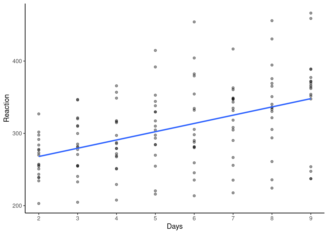
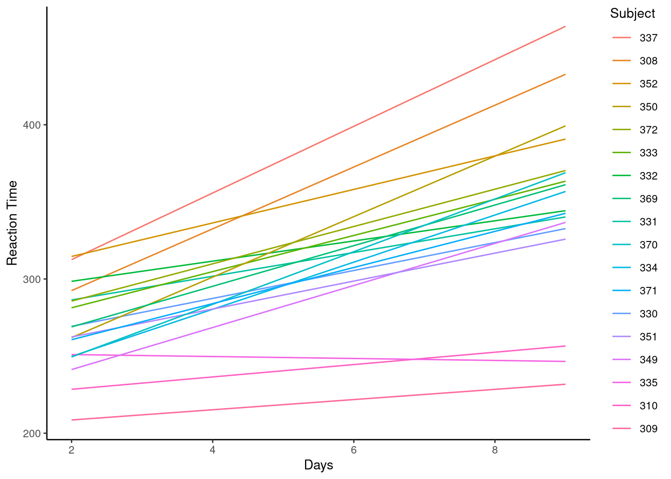
Figure 11.1: Reaction time plotted as a function of days without sleep from the sleepstudy data set.
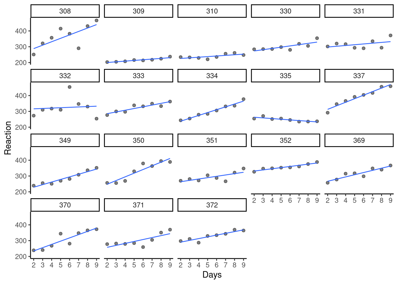
Now let’s have a look at the trends of Reaction over time, across all participants. This is shown in Figure 11.1. We see that, overall, as might be expected, as days without sleep increase, so too does participants’ reaction time, starting at around 260ms at baseline (day 2) and finishing at around 350ms on day 9. However, although looking at the overall trend across all participants is illuminating for us, do you think it is reasonable, or nuanced? In other words, would we expect all participants to follow this same trend in reaction time, or is it more reasonable to think that some participants might be faster or slower at baseline and that the effects of sleep deprivation might be different for all participants? Let’s take a look at the plot of reaction time over time, but this time faceting the plot by participant, i.e., creating a plot per participant, see Figure 11.2. This plot gives us some quite clear answers. Although several participants follow the broad trend described above, e.g., participants 333, 334 and 349, we see several who do not, e.g., the baseline reaction time for participant 309 is around 200ms and only rising slightly to 250ms across the duration of the study. In addition, the reaction time for participant 335 is around 250ms at baseline but then proceeds to decrease over time. What this tells us, then, is that there is variation across participants regarding their baseline reaction time, and the rate of change in their reactions over time.
Figure 11.2: Reaction time plotted as a function of days without sleep from the sleepstudy data set. Each subplot represents the data from one subject.
Bearing in mind what we’ve seen in Figure 11.2, let’s think about how we would model the data, using the tools we currently have at our disposal. An obvious choice of model to use to begin to understand this dataset would be a normal linear model predicting reaction time from days sleep deprived, i.e., trying to understand the impact on reaction time by days of sleep deprivation. Let’s revisit the formal definition of that model: \[
y_i \sim N(\mu_i, \sigma^2), \quad \mu_i = b_0 + b_1x_i, \quad \text{for } i \in 1, \ldots, n.
\]
Recall that this definition assumes that every observation of our outcome variable (\(y_i\)) is drawn from a normal distribution with some unknown mean (\(\mu_i\)) and variance (\(\sigma^2\)). We assume that the mean (\(\mu_i\)) is a linear combination of the intercept (\(b_0\)) and the slope term, for a given value of the predictor (\(b_1x_i\)), and that this formula applies for each observation in the dataset (\(i \in 1, \ldots, n\)). Applying this model to the sleepstudy data, we would be aiming to estimate the mean and variance of reaction time, for a given day without sleep, for the population.
You may recall from Chapter 10 that repeated-measures ANOVA can handle data with multiple observations per participant by modelling participants as a within-subject factor. However, that approach assumes categorical predictors (for example, day 1 vs day 2 vs day 3) and a constant pattern of covariances between repeated measures — an assumption known as sphericity. In the sleepstudy data, our predictor Days is continuous, and we may expect each participant’s trajectory over time to differ in both their starting point and rate of change. So, while repeated-measures ANOVA can capture non-independence for categorical time points, it is not appropriate for this continuous predictor.
At this point, the only tool we have for handling a continuous predictor is the standard linear model. We know that the observations are grouped within participants, but this model cannot account for that dependency. Nevertheless, let’s go ahead and fit the linear model to the data and examine the coefficients.
M_11_1 <-lm(Reaction ~ Days, data = sleepstudy)tidy(M_11_1)
# A tibble: 2 × 5
  term        estimate std.error statistic  p.value
  <chr>          <dbl>     <dbl>     <dbl>    <dbl>
1 (Intercept)    245.      11.0      22.2  4.11e-48
2 Days            11.4      1.85      6.18 6.32e- 9
So, using this model, we have estimated that in the population, reaction time at baseline (\(b_0\)) is 245ms and increases linearly (\(b_1x_i\)) by 11.4ms for every additional day an individual experiences sleep deprivation. However, we have generated these estimates by using a model that has ignored the fact that the observations in our sample come from not one individual, but from multiple individuals; in other words, we have omitted that the observations or measurements provided by an individual participant are uniquely impacted by that individual, they are not independent of each other and that certain observations belong to certain individuals.
What we can do, then, is think about this structure of data as having different levels, with the lowest level of the hierarchy, here the reaction times, being level 1 and the next level, the participant, being level 2. We would say of this example that level 1 is nested within level 2, that reaction time is nested within participant.
Hierarchies exist extensively in social science data. A classic example is that of an educational setting. Imagine in a university there are 500 students enrolled on a course and that this group of 500 is split into 50 groups of 10, each with a different tutor, to learn a specific skill, let’s say linear algebra, and they take a test at the end of the course to assess their learning. Although there will be a high degree of standardisation in the materials, teaching methods, etc., the students’ outcomes will be uniquely impacted by the group in which they are placed — for example, the skill of the tutor is likely to vary, and the peer-to-peer support is likely to change from group to group. Such contextual factors as these mean that the students’ outcomes (level 1 of the hierarchy) are uniquely impacted by the group to which they are allocated (level 2 of the hierarchy), as such outcomes are not independent, they are nested within group.
It is not uncommon in social science research to see many layers of hierarchy — for example, school children’s educational outcomes (level 1) are influenced by the classroom in which they are taught (level 2), which may in turn be influenced by their school (level 3), which in turn may be influenced by the school district (level 4). In this chapter, however, we will only focus on modelling a hierarchy with two levels.
11.2 Strategies for handling data hierarchies
There are several strategies for dealing with hierarchies in data. We will outline these below, run them using the sleepstudy data and discuss the strengths and limitations of each technique, ending finally with our recommended approach, multilevel modelling.
11.2.1 Option 1: Ignore the hierarchy
When we modelled the sleepstudy data using a normal linear model, we ignored the hierarchy in the data. We did not reference anywhere in the model that our data had a hierarchical structure, that observations were not independent and were in fact influenced by the participant who generated them. This is an example of complete pooling, whereby level 2 of the hierarchy is ignored and only the measurements at level 1 are modelled.
The issue with this approach is that one assumption of a linear model is independence of observations — observations in sleepstudy are clearly not independent (nested within participant) — therefore we are running a model that makes assumptions that we clearly know are wrong. A consequence of this erroneous assumption is that we overestimate our certainty in the inferences of our parameters by saying that we have, in the sleepstudy data, 144 independent data points, when in fact we have 18 groups of intercorrelated data with 8 data points each.
11.2.2 Option 2: Aggregate the data
Another way in which hierarchies are managed is through collapsing rows of data, also called aggregation and is seen frequently in experimental studies when participants are required to respond to multiple trials. For example, imagine an experiment that was designed to measure 100 participants’ anxiety in response to pictorial stimuli. One participant may be presented with, say, 5 high-anxiety images and 5 low-anxiety images and asked to respond to each image on some anxiety rating scale of 1-10, leading to 10 anxiety measures, 5 in each condition, as represented in the data below:
pp_1_df <-tibble(pp =rep(1, 10),condition =rep(c("high", "low"), each =5, times =1),score =c(8, 9, 6, 7, 8, 2, 3, 4, 1, 2))pp_1_df
# A tibble: 10 × 3
      pp condition score
   <dbl> <chr>     <dbl>
 1     1 high          8
 2     1 high          9
 3     1 high          6
 4     1 high          7
 5     1 high          8
 6     1 low           2
 7     1 low           3
 8     1 low           4
 9     1 low           1
10     1 low           2
Often, an approach to dealing with this data is to aggregate the 5 scores for each condition, resulting in a mean high-anxiety image score and a mean low-anxiety image score, for each participant:
# A tibble: 2 × 2
  condition pp1_score
  <chr>         <dbl>
1 high            7.6
2 low             2.4
It is then these aggregated scores that are modelled rather than the raw scores for each image.
This is promlematic since aggregating data in this way loses lots of information per participant — for example, if 100 participants each gave us 5 measurements across two conditions, we would have a total of 1000 observations, 500 for each condition. Aggregating those to a mean score for each condition for each participant would lead to just 100 measurements, 50 per condition. Aggregating the data effectively means that we are losing data, and specifically losing information around participant variance.
11.2.3 Option 3: One model per participant
Turning back to our sleepstudy data, we may decide to manage the hierarchy by running one model per participant in the dataset. By doing this, we are explicitly recognising that the reaction times are nested within each participant and therefore generating estimates of parameters per participant. This could be achieved practically by including a term in a linear model that fits a model per participant and is an example of a no pooling approach whereby all estimates about groups in level 2 of the hierarchy are inferred independently. When we include Subject in this model this way, we can term it a fixed effect.
M_11_2 <-lm(Reaction ~0+ Subject + Subject:Days, data = sleepstudy)
In a model specified like this we do not derive a single population intercept and slope, but rather an intercept and slope estimate for each participant in the study. Immediately this model represents an improvement on our complete pooling approach as level 2 of the hierarchy is included in the model, i.e., we are not ignoring that it exists. A consequence of this is that we now have varying estimates of intercepts and slopes for each individual, which matches our expectation of heterogeneity in individuals’ baseline reaction times and variability in the (linear) effect of sleep deprivation.
Although this approach may feel like a complete solution to managing hierarchies in the data, there is one major problem. This model essentially assumes eighteen independent datasets, one per participant, each with a resulting intercept and slope term. In many cases, but not all, the estimates of the individuals in the sample are not of substantive interest to us so the results of this no pooling model might be interesting, but they do not immediately tell us about the wider population beyond this sample, which is usually the target of our analysis. As such, this is the biggest failing of the no pooling approach: we cannot generalise the results beyond the individuals in the sample.
11.2.4 Option 4: Multilevel models
As noted above, there are many ways of handling hierarchies in data, many of which are sub-optimal. Here we turn to our recommended approach, and the focus of this chapter, multilevel models. Multilevel models are so-called since they are models of models — we create a model for each of the different groups in our data (e.g., each participant in the sleepstudy data) and then model the variability of these models across that group. Multilevel models improve on all of our approaches to managing data hierarchies outlined above in that groups can be accounted for in the model, no aggregation of data is needed and estimates from the model can be used to generalise beyond the sample. An additional benefit of multilevel models is that we can have hypotheses about our data at all or any level of the hierarchy. In our sleepstudy example, our hypothesis was situated at level 1, regarding the reaction times — we weren’t necessarily interested in a given participant’s reaction time, or the variability of participants’ reaction times around the population average. However, in a multilevel model, we have the option of evaluating the impact of participant, of level 2 in the hierarchy. This might be more valuable in some research paradigms than in others — for example, in an education setting, there may be substantive interest in whether certain classrooms (level 2) perform better on a given measurement (level 1) than others, or when deciding on stimuli to use in a study it might be important to know if some stimuli (level 2) yield very different responses (level 1) as compared to others.
There are many varieties of multilevel models, here we will focus on just two linear variants: random intercept only and random intercept and random slope models. We will also only be focusing on nested data, such as those in the sleepstudy data — other forms of hierarchies exist (e.g., crossed structures) but will not be considered here.
11.3 Random intercept multilevel linear models
First we will look at the formal definition of a random intercept multilevel model. This might look daunting on first inspection, but as we work through it line by line, you’ll see the similarities to the normal linear model — remember, as we noted at the start of this chapter, multilevel models are extensions of the normal linear model, so you’ll already have much of the knowledge needed to tackle these models.
The first two lines of this model are very similar to the normal linear model. We see that each observed value of \(y\) is a sample from a normal distribution (\(y_i \sim N(\mu_i, \sigma^2)\)), whose mean is \(\mu_i\) and whose variance is \(\sigma^2\). The mean \(\mu_i\) is a linear combination of the intercept \(\beta_{0j}\) and slope coefficient \(\beta_{1}\) for a given level of \(x_i\). Note, though, that the notation for the intercept is different to the normal linear model as here it has subscript \(j\). This subscript \(j\) refers to a given group in level 2 of the hierarchy — in the sleepstudy data, that is for a given participant in the sample of participants. What this means, then, is that in the multilevel model, each group in level 2 of the hierarchy (each participant) will have their own intercept. Line three of the model tells us how this intercept is defined: it is the population intercept (\(\beta_{0}\)) plus \(\zeta_{0j}\) (zeta), where \(\zeta_{0j}\) is the difference between a given participant’s intercept and the population intercept, the offset, or residual. As such, in this model, we fit an intercept per each group in the level 2 hierarchy (participant) which is calculated from their offset from the population intercept. The fifth line of the model tells us that we expect the vector of the intercept offsets for each group in level 2 (all participants) \(\zeta_{0j}\) to follow a normal distribution with mean zero and variance \(\tau_0^2\). The term \(\tau_0\) (tau) is therefore the standard deviation of the random intercepts, describing how much participants vary around the population intercept. In other words, larger values of \(\tau_0\) indicate greater between-participant variation in baseline reaction times. Looking back at line 3, we do not see the \(j\) subscript associated with the slope coefficient and, as is clarified in line 4, the population slope term is equal to the inferred slope term of the model — in other words, the slope term does not vary by level 2 groups.
There is a lot to dissect there: the key thing to take away at this point is that the multilevel model is similar to the normal linear model – we still estimate a population intercept and slope but in addition we also estimate intercepts for each group in level 2 which we calculate using the offsets from the population intercepts.
Let’s look at the random intercept multilevel linear model visually using the sleepstudy data. In a simple linear model (with complete pooling), we estimate a single intercept representing the average baseline reaction time for the population and a single slope representing the average change in reaction time across days. This model ignores the fact that reaction times are grouped within participants and therefore not independent.
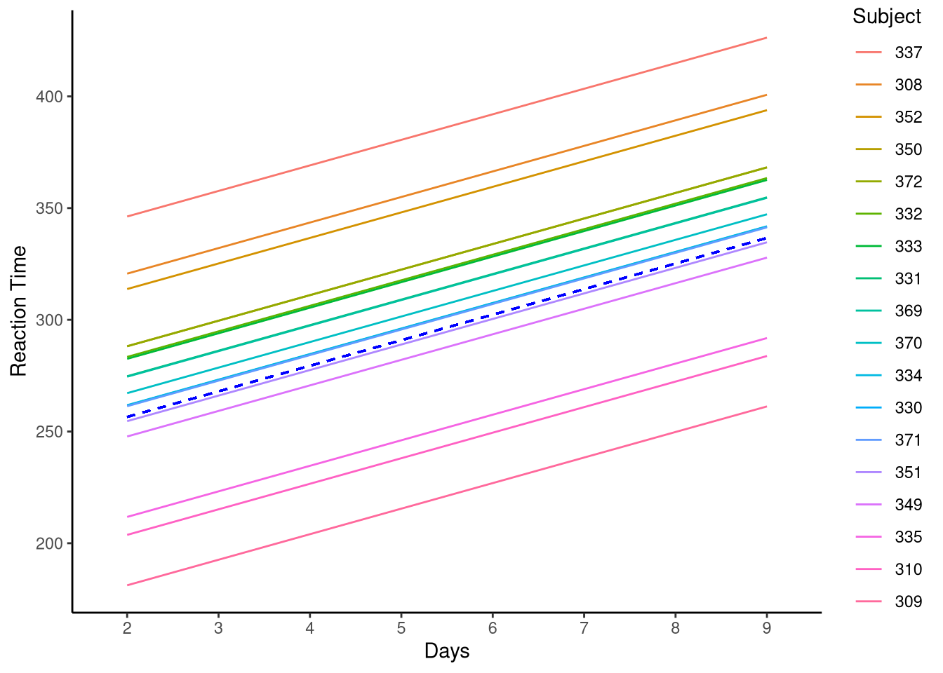
In the random intercept multilevel model, we extend this by allowing each participant to have their own intercept — that is, their own baseline level of reaction time — while retaining a common slope across all participants. This relaxes the assumption that everyone starts at the same level while still assuming the same rate of change over time. The resulting models are shown in Figure 11.3, where the dotted line represents the population (complete pooling) model and the coloured lines represent participant-specific intercepts estimated by the multilevel model for a sample of five participants.
Figure 11.3: Varying intercept model for a sample of five participants.
Finally, it may also help your understanding to see the random intercept multilevel model expressed using the formula for a straight line:
\[Y_{ij} = b_0 + \zeta_{0j} + b_1X_{ij} + \varepsilon_{ij}\] This model shows us that the predicted value of the outcome for a given observation in a given group in the level 2 hierarchy (i.e., participant) is a linear combination of the population intercept plus the level 2’s offset from the population intercept plus the slope term multiplied by the value of the predictor of interest. The final term represents the residual error for each observation — the deviation of an individual measurement from its group’s fitted line.
11.3.1 Random intercept multilevel linear model using R
Note 11.1: How multilevel models are estimated: Maximum likelihood
Up to this point, our linear models have been estimated using ordinary least squares (OLS), which finds the parameter values that minimise the residual sum of squares (RSS):
For multilevel models, OLS no longer works well because we have multiple sources of variance — within groups (level 1) and between groups (level 2). Instead, these models are estimated using maximum likelihood (ML) or restricted maximum likelihood (REML).
The idea of maximum likelihood is to choose the parameter values that make the observed data most probable under the model:
where \(\theta\) represents the model parameters (e.g., fixed effects and variance components). The likelihood function ($L(| y) $) can be thought of as a score of how well a particular set of parameters explains the observed data: higher values indicate a better fit. In practice, when we run the model in R, the computer searches for the values of \(\theta\) that maximise this likelihood.
Under maximum likelihood (ML), all parameters — both fixed effects (like \(b_0\) and \(b_1\)) and random effects (variance components such as \(\tau^2\) and \(\sigma^2\)) — are estimated together. This can lead to slightly biased estimates of the variance components because ML does not account for the fact that the fixed effects were estimated from the same data.
Restricted maximum likelihood (REML) addresses this by first removing the influence of the fixed effects before estimating the variance components. By focusing only on the part of the data that reflects random variation, REML produces less biased and more stable estimates of the variances, especially in smaller samples. The fixed effects are then estimated in the usual way, conditional on those variance estimates.
You don’t need to work through the maths here, but it’s useful to know that the fixed effects (\(b_0, b_1\)) and the variance components (\(\tau^2\), \(\sigma^2\)) all come from the likelihood framework rather than least squares. Conceptually, though, both approaches share the same goal: to find the model that best fits the data.
To implement the model in R, we’ll use the lmer() function from sgsur (which is a reexport from the lmerTest package, which itself is an extension of the lme4 package) and keep using our sleepstudy data from which we are trying to understand the effect of sleep deprivation over time on reaction times. For this model, the outcome variable is Reaction and the predictor is Days, and we need to tell the model that observations are nested or grouped under Subject and hence to estimate an intercept per level of Subject, i.e., per participant — we do so using the following syntax:
M_11_3 <-lmer(Reaction ~ Days + (1|Subject), data = sleepstudy)
The syntax should feel quite familiar; the only new additions we have are that we use the function lmer rather than lm and the term (1|Subject). It is the (1|Subject) term that tells the model to estimate an intercept per level of Subject — this is often called a random intercept, or more broadly a random effect. The right-hand side of the pipe | tells the model to vary intercepts by Subject, the left-hand side tells the model to keep the slope constant for all participants. In other words, in this model we are assuming that participants’ baseline reaction time is variable, but that their rate of change is constant — this may or may not be a sensible assumption to make, but we’ll come back to this later. Let’s take a look at the output:
summary(M_11_3)
Linear mixed model fit by REML. t-tests use Satterthwaite's method [
lmerModLmerTest]
Formula: Reaction ~ Days + (1 | Subject)
   Data: sleepstudy

REML criterion at convergence: 1430

Scaled residuals:
    Min      1Q  Median      3Q     Max
-3.6261 -0.4450  0.0474  0.5199  4.1378

Random effects:
 Groups   Name        Variance Std.Dev.
 Subject  (Intercept) 1746.9   41.80
 Residual              913.1   30.22
Number of obs: 144, groups:  Subject, 18

Fixed effects:
            Estimate Std. Error      df t value Pr(>|t|)
(Intercept)  245.097     11.829  30.617   20.72   <2e-16 ***
Days          11.435      1.099 125.000   10.40   <2e-16 ***
---
Signif. codes:  0 '***' 0.001 '**' 0.01 '*' 0.05 '.' 0.1 ' ' 1

Correlation of Fixed Effects:
     (Intr)
Days -0.511
First in the output, we have information about our residuals. Recall that residuals are the difference between the observed value and the predicted value; we expect them to be centred on zero and approximately normally distributed (see Note 7.1). Next, we’ll skip to the fixed effects — remember that these are the effects that we assume are constant for the population. These are formatted similarly to results in a normal linear model and can be interpreted the same way: we have estimates of the intercept and slope, along with standard errors of these estimates and t-values. We can also obtain the 95% confidence intervals of the intercept and slope using the confint() function:
The fixed effects show us that on average, in the population, an individual’s baseline reaction time is 245.1ms and that for every day that individual experiences sleep deprivation, their reaction time will increase by 11.44ms. These estimates are the same as those from a complete pooling model of the data. However, this equivalence holds only because each participant contributes the same number of observations. If some participants had more or fewer measurements, the multilevel model would give greater influence to participants with more data and partially pull (shrink) estimates from participants with fewer data toward the population average (see Note 11.2). In contrast, a complete pooling model ignores these differences and treats every observation as equally independent. This is another advantage of multilevel modelling: it can handle unbalanced or missing data without requiring any cases to be deleted from the analysis.
Note 11.2: Shrinkage: borrowing strength across groups
One of the most powerful features of multilevel models is shrinkage. When each group in the data (e.g., participant) has its own intercept or slope, the model balances two sources of information: - the group’s own data, and - the overall population trend.
Groups with many observations provide strong evidence about their own intercepts and slopes, so their estimates remain close to their sample means. Groups with few observations provide weaker evidence, so their estimates are pulled (“shrunk”) toward the population mean. This prevents noisy, data-sparse groups from having extreme or unreliable estimates and leads to more stable overall inferences.
Shrinkage is a natural consequence of fitting a hierarchical model — no extra step or correction is required. It is what allows multilevel models to “borrow strength” across groups while still capturing meaningful between-group variation.
Looking at the random effect section of the output we have a column named Groups under which we see our level 2 grouping variable, Subject. Reading across this row we see a value for variance which is the variance attributable to the variability across the participant intercept offsets — in other words, this value tells us how much variance in the model is captured by the level 2 intercept offsets — the square root of this is also shown, giving us this information in the form of a standard deviation (\(\tau_0\)). We can interpret the standard deviation here in the typical way: a larger standard deviation indicates that the intercepts were relatively spread out, and a smaller standard deviation indicates that they were closer together. More informatively, though, we can use this standard deviation in conjunction with the fixed effect intercept estimate, \(b_0\), to say that intercepts across all participants in the population are estimated to be normally distributed around \(b_0\), the population intercept, with a standard deviation of \(\tau_0\). From this, we can calculate the approximate 95% range of intercepts in the population using the following: \[
b_0 \pm 1.96 \times \tau_0.
\] As such, we find that 95% of intercepts in the population will range between 163.17ms and 327.02ms.
The following row shows the residual variance (and standard deviation), that is, any variance in the model that is left unexplained. We can see from these numbers that the variance accounted for by including a random intercept, i.e., letting each participant have a different baseline reaction time, is nearly twice that of the residual variance in the model. This tells us that most of the variation in reaction times arises from stable differences between participants rather than from random fluctuation within participants over time.
Next, we can look at the values of the intercepts for each participant in the sample, confirming that they are varying for the different levels of the level 2 variable, and noting that the slope term is constant for all participants:
Finally, as we have done in previous chapters, we can make predictions easily using the predict() function. Here, the crossing() function creates all combinations of Days (from 2 to 9) and Subject, so that we generate predictions for every participant at each day included in the study.
A question we might have at this point, and one which we alluded to earlier in the chapter, is whether the assumption that the effect of sleep deprivation is constant for all participants is a reasonable one. To illustrate this, let’s overlay the intercept only model estimates over the raw data points, faceted by participant:
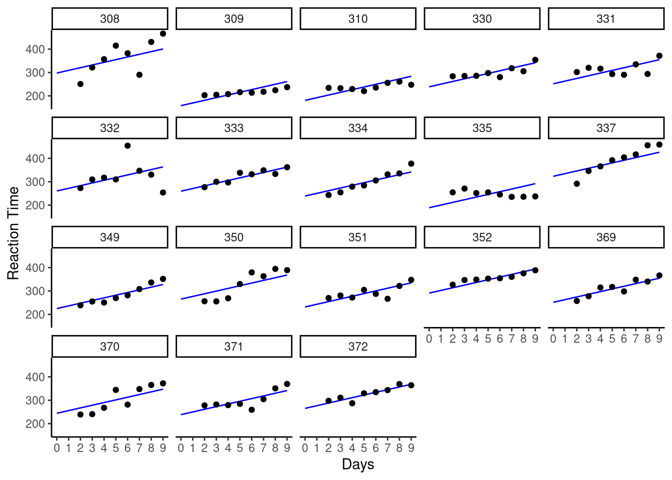
Figure 11.4: Random intercepts only model fits superimposed on original data.
We see that by allowing the intercept to vary per participant, it seems to relatively accurately represent the baseline reaction time for the participants. We also see that the slope of the line captures the effect of sleep deprivation over time well for some participants, e.g., 369 and 372. However, we also see that this fixed slope effect does not capture the effect well for other participants, e.g., 308 or 335. As we noted earlier in the chapter, this heterogeneity in the effect of sleep deprivation over time makes theoretical sense too. As such, we can run another multilevel model variant: the random intercept and random slope multilevel linear model.
11.4 Random intercept and random slope multilevel linear model
In our previous model, we allowed the intercepts to vary per group in the level 2 hierarchy (participant) but fixed the slopes to be constant. There are likely to be instances, however, when assuming a constant slope, or rate of change, across groups in the level 2 hierarchy is not reasonable. In this section, we will look at the random intercept and random slope multilevel model, starting with the formal model definition:
This is almost identical to the random intercepts model. Indeed, we still see that the intercept varies by the level 2 group as denoted by the subscript \(j\), but in addition, we now have subscript \(j\) next to \(\beta_1\), our slope coefficient, meaning that in this model, we assume a different slope for each group in the level 2 hierarchy. The fourth line tells us that this slope is a linear combination of the population slope \(b_1\) plus a given group of level 2’s offset, or difference, from this (\(\zeta_{1j}\)).
A visualisation of this model is shown in Figure 11.5 for a sample of five participants.
Figure 11.5: Random slopes and intercepts model fits for a sample of five participants. Each coloured line represents a participant’s fitted regression line showing predicted reaction times across days of sleep deprivation. Both intercepts and slopes vary across participants, allowing each person to have their own baseline reaction time and their own rate of change over days.
Each coloured line represents a participant’s fitted regression line, showing their predicted reaction times across days. Unlike the previous plot, where only the intercepts varied, here both the intercepts and the slopes differ across the sampled participants. This means each participant has their own baseline level and their own rate of change in reaction time over days of sleep deprivation.
We can also conceptualise the model using the formula for a straight line: \[
Y_{ij} = b_0 + \zeta_{0j} + (b_{1} + \zeta_{1j})X_{ij}
\]
This shows that the predicted value of the outcome for a given observation in a given group in the level 2 hierarchy (participant) is a linear combination of the population intercept plus the participant’s offset from that intercept, together with the population slope plus the participant’s offset from that slope, multiplied by the value of the predictor of interest.
11.4.1 Random intercept and random slope multilevel linear model using R
Running this model in R only requires a slight adjustment of the syntax we used for the random intercepts model. We now replace the constant term 1 on the left-hand side of the pipe with the variable by which we want slopes to vary.
M_11_4 <-lmer(Reaction ~ Days + (Days|Subject),data = sleepstudy)
Let’s take a look at the model output:
summary(M_11_4)
Linear mixed model fit by REML. t-tests use Satterthwaite's method [
lmerModLmerTest]
Formula: Reaction ~ Days + (Days | Subject)
   Data: sleepstudy

REML criterion at convergence: 1404.1

Scaled residuals:
    Min      1Q  Median      3Q     Max
-4.0157 -0.3541  0.0069  0.4681  5.0732

Random effects:
 Groups   Name        Variance Std.Dev. Corr
 Subject  (Intercept) 992.69   31.507
          Days         45.77    6.766   -0.25
 Residual             651.59   25.526
Number of obs: 144, groups:  Subject, 18

Fixed effects:
            Estimate Std. Error      df t value Pr(>|t|)
(Intercept)  245.097      9.260  16.999  26.468 2.95e-15 ***
Days          11.435      1.845  17.001   6.197 9.74e-06 ***
---
Signif. codes:  0 '***' 0.001 '**' 0.01 '*' 0.05 '.' 0.1 ' ' 1

Correlation of Fixed Effects:
     (Intr)
Days -0.454
We interpret the model output in the same way as the random intercept model, so we will not cover that in detail here, but instead we’ll draw our attention to two additional pieces of information in the output. First, in the random effects section, we now see a row relating to Days — we interpret this the same as we did for Subject and can see the variance associated with the varying slope term and its square root term, the standard deviation. Again, we can use this standard deviation in conjunction with the fixed effect slope estimate, \(b_1\), to say that slopes across all subjects in the population are estimated to be normally distributed around \(b_1\), the population slope, with a standard deviation of \(\tau_1\). From this, we can calculate the approximate 95% range of slopes in the population as follows: \[
b_1 \pm 1.96 \times \tau_1
\] As such, we find that 95% of slopes in the population will range between -1.83ms and 24.7ms.
Staying in the random intercepts section, let’s take a look at the value -0.25 under the heading Corr. This value shows the correlation between the random intercept and random slope terms. In the context of the sleepstudy data, this value would allow us to understand the relationship between baseline reaction time and the impact of sleep deprivation.
Finally, we can make predictions as usual using the model with the predict() function:
Daniel B. Wright’s “Modelling clustered data in autobiographical memory research: the multilevel approach” (Wright, 1999) provides a clear introduction to multilevel modelling for cognitive and psychological data, demonstrating how to handle dependencies in clustered observations.
Baayen et al.’s “Mixed-effects modelling with crossed random effects for subjects and items” (Baayen et al., 2008) introduces crossed random effects for observations nested within multiple grouping factors, explaining why both participant and item variability must be modelled to avoid inflated Type I error rates.
Judd et al.’s “Treating stimuli as a random factor in social psychology” (Judd et al., 2012) addresses the long-standing issue of stimuli being treated as fixed when they should be modeled as random, providing a comprehensive solution to this pervasive problem.
11.6 Chapter summary
Multilevel (mixed-effects) models extend the general linear model to data with hierarchical or clustered structure, where observations are nested within groups such as repeated measures within individuals or students within schools.
Complete pooling ignores group structure entirely, no pooling estimates separate parameters per group, and partial pooling (multilevel modelling) borrows strength across groups while allowing group-specific deviations from population trends.
Random intercept models allow each group to have its own baseline level while assuming all groups share the same slope, capturing between-group heterogeneity in outcome levels.
Random slope models further allow the effect of a predictor to vary across groups, capturing between-group heterogeneity in both baseline levels and predictor effects simultaneously.
Shrinkage (partial pooling) stabilises group-level estimates by pulling extreme estimates toward the population mean, with stronger shrinkage for groups with fewer observations or more uncertain estimates.
Maximum likelihood (ML) and restricted maximum likelihood (REML) are estimation methods for multilevel models, with REML preferred for estimating variance components and ML used when comparing models with different fixed effects.
Fixed effects represent population-average relationships between predictors and outcomes, while random effects capture group-specific deviations from those population averages, modelled as draws from a distribution.
The lmer() function in R specifies multilevel models using formula notation with vertical bars separating fixed effects from random effects, allowing random intercepts (1 | group) and random slopes (predictor | group).
Intraclass correlation (ICC) quantifies the proportion of total variance attributable to between-group differences, indicating the degree of clustering and the necessity of multilevel modelling.
Multilevel models unify repeated-measures ANOVA, hierarchical regression, and growth curve analysis under one framework, handling unbalanced data and providing principled inference for clustered observations.
Baayen, R. H., Davidson, D. J., & Bates, D. M. (2008). Mixed-effects modeling with crossed random effects for subjects and items. Journal of Memory and Language, 59(4), 390–412. https://doi.org/10.1016/j.jml.2007.12.005
Belenky, G., Wesensten, N. J., Thorne, D. R., Thomas, M. L., Sing, H. C., Redmond, D. P., Russo, M. B., & Balkin, T. J. (2003). Patterns of performance degradation and restoration during sleep restriction and subsequent recovery: A sleep dose-response study. Journal of Sleep Research, 12(1), 1–12. https://doi.org/https://doi.org/10.1046/j.1365-2869.2003.00337.x
Judd, C. M., Westfall, J., & Kenny, D. A. (2012). Treating stimuli as a random factor in social psychology: A new and comprehensive solution to a pervasive but largely ignored problem. Journal of Personality and Social Psychology, 103(1), 54–69. https://doi.org/10.1037/a0028347