library(tidyverse)
library(sgsur)9 ANOVA and general linear models
In the previous chapters, we explored linear regression models where our predictor variables were continuous, such as GDP per capita or life expectancy. This chapter extends our modelling toolkit to handle categorical predictors, variables that divide observations into distinct groups or categories rather than taking on a continuous range of values. When we use categorical predictors in statistical analysis, we often frame our research questions in terms of comparing means across groups, and use techniques collectively known as Analysis of Variance (ANOVA).
ANOVA might initially seem like a completely different statistical technique from the regression methods we’ve been studying. Traditionally, ANOVA is taught as a method for comparing group means, while regression is presented as a way to model relationships between variables. However, this apparent distinction is largely artificial. As we’ll discover in this chapter, ANOVA is actually a special case of linear regression where the predictors happen to be categorical rather than continuous. This unified perspective, known as the general linear model, provides a powerful framework that encompasses both regression and ANOVA as different faces of the same underlying mathematical approach.
The general linear model framework offers several advantages over treating ANOVA and regression as separate techniques. First, it allows us to seamlessly combine categorical and continuous predictors in the same model, enabling us to answer more sophisticated research questions. Second, it provides a consistent set of tools and interpretive strategies across different types of analyses. Most importantly, understanding this connection deepens our grasp of both methods and reveals the elegant mathematical unity underlying much of applied statistics.
Throughout this chapter, we’ll begin with one-way ANOVA, which is the comparison of means across multiple groups defined by a single categorical variable. We’ll then extend this to factorial ANOVA designs that examine multiple categorical factors simultaneously, including their potential interactions. Finally, we’ll demonstrate how to combine categorical and continuous predictors in mixed models. By the end of this chapter, you’ll see that whether we call our analysis “ANOVA” or “regression” depends more on our perspective and emphasis than on any fundamental mathematical differences.
The chapter covers
- Analysis of variance partitions total variation into between-group and within-group components to test whether categorical predictors explain meaningful differences.
- ANOVA is a special case of linear regression where predictors are categorical, unified under the general linear model framework.
- Dummy coding represents categorical variables as binary indicators, with coefficients interpretable as differences from a reference category.
- Pairwise comparisons with adjustments like Tukey’s HSD control family-wise error rates when testing multiple group differences.
- Factorial designs with multiple categorical predictors reveal main effects and interaction effects that capture non-additive relationships.
- Types of sums of squares (I, II, III) differ in how they partition variance, particularly mattering for unbalanced designs or when interactions are present.
9.1 One-way ANOVA
The gss2021 dataset in sgsur provides a subset of variables from the 2021 edition of the General Social Survey (GSS). The GSS is a nationally representative survey conducted by the University of Chicago that has tracked American social attitudes, behaviours, and demographic characteristics since 1972. In Figure 9.1, using the gss2021 dataset, we show boxplots of the logarithm (base 10) of personal income (lincome) for each of five groups of people, defined by their level of education (degree). The levels of education are less than high school (<HS), high school (HS), junior college (JrColl), university undergraduate degree (BA), and post-graduate degree (Grad). We use the log of income (lincome) rather than income itself as the outcome variable given that income is highly right skewed but its log transform is closer to symmetrical and bell-shaped.
tukeyboxplot(y = lincome, x = degree, data = gss2021)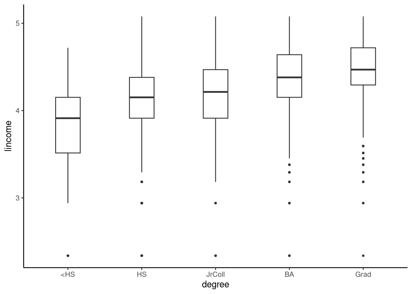
The means, standard deviations of lincome and the number of individuals in each group can be obtained as follows:
summarise(gss2021,
          avg = mean(lincome),
          stdev = sd(lincome),
          n = n(),
          .by = degree) |>
  arrange(degree)
# A tibble: 5 × 4
degree avg stdev n
<fct> <dbl> <dbl> <int>
1 <HS 3.77 0.569 77
2 HS 4.09 0.494 877
3 JrColl 4.14 0.473 249
4 BA 4.32 0.468 713
5 Grad 4.44 0.448 528From Figure 9.1 and the descriptive statistics, the distributions of income across different education levels clearly appear to differ: as education level increases, income distributions shift toward higher values. However, each education group represents only a sample from the broader population of Americans with that level of education. If we drew new samples from these populations, we would obtain different distributions of lincome. This means the sample means for lincome in each group are estimates of the unknown population means, not the true population values themselves. As in the previous chapters, we can use statistical inference to draw conclusions about these population means based on our sample data.
9.1.1 Statistical model
To conduct statistical inference, we begin by specifying a statistical model for how the data were generated. A common assumption, which extends the independent samples t-test model from Section 6.5, is that each education group is drawn from a normal distribution. These five normal distributions have different means, but we commonly make the default assumption that they share the same (unknown) standard deviation. Given this assumed model, we can apply the same inferential methods from previous chapters to test hypotheses and construct confidence intervals for the population means. This analysis is called a one-way ANOVA, where ANOVA stands for analysis of variance. More precisely, one-way ANOVA refers to a specific null hypothesis test within this statistical framework, which is an example of the broader class of methods known as general linear models.
In a one-way ANOVA, we work with \(J\) distinct groups of data, where each group represents a different level or condition of a single categorical predictor variable. In the context of ANOVA, the categorical predictor variables are often referred to as factors. Within group \(j\), we have \(n_j\) individual observations. For example, if we label the five groups <HS, HS, JrColl, BA, Grad as groups 1 to 5, the sample sizes are \(n_1 =77\), \(n_2 =877\), \(n_3 =249\), \(n_4 =713\), \(n_5 =528\). We denote the \(i\)-th observation from group \(j\) as \(y_{ji}\). This double subscript system allows us to keep track of both which group an observation belongs to (first subscript) and its position within that group (second subscript), providing the organisational structure necessary for the subsequent mathematical analysis.
The fundamental assumption underlying one-way ANOVA is that for each group \(j \in \{1,2\ldots J\}\), the observations follow a normal distribution with a group-specific mean but common variance: \[ y_{ji} \sim \textrm{N}(\mu_j,\sigma^2) \quad \text{for $i \in \{1,2 \ldots n_j\}$} \] This distributional assumption can be expressed in several equivalent mathematical forms, each offering different insights into the structure of the model. The first alternative representation expresses each observation as the sum of its group mean and a random error term: \[y_{ji} = \mu_j + \epsilon_{ji}, \quad \text{where $\epsilon_{ji} \in N(0, \sigma^2)$}\] This formulation makes explicit the additive nature of the error and highlights how individual observations deviate randomly from their group means.
A third equivalent representation introduces the concept of an overall grand mean and group-specific deviations from this grand mean: \[y_{ji} = \mu + \alpha_j + \epsilon_{ji}, \quad \text{where $\epsilon_{ji} \in N(0, \sigma^2)$}\]
In this parameterisation, \(\mu\) represents the grand or overall mean across all groups, and \(\alpha_j = \mu_j - \mu\) represents the deviation of group \(j\)’s mean from the overall mean. This formulation proves particularly useful for understanding how ANOVA decomposes variation and for connecting ANOVA to regression analysis.
The core insight of analysis of variance lies in its ability to partition the total variation in the data into meaningful components that can be attributed to different sources. This partitioning forms the basis of all hypothesis testing in ANOVA and represents one of the most elegant concepts in statistical analysis.
The total variation in the data can be mathematically decomposed as follows: \[ \underbrace{\sum_{j=1}^J\sum_{i=1}^{n_j} (y_{ij}-\bar{y})^2}_{\text{Total}} = \underbrace{\sum_{j=1}^J n_j (\bar{y}_j-\bar{y})^2}_{\text{Between}} + \underbrace{\sum_{j=1}^J\sum_{i=1}^{n_j} (y_{ij}-\bar{y}_j)^2}_{\text{Within}} \]
In this decomposition, \(\bar{y}_j\) represents the mean of group \(j\), and \(\bar{y}\) represents the overall mean of all data points. The three components of this equation tell a complete story about the sources of variation in the data. The total sum of squares (on the left side) captures all variation in the data by measuring how much each individual observation deviates from the overall mean. The between-groups sum of squares captures variation that can be attributed to differences between group means, weighted by the number of observations in each group. The within-groups sum of squares captures variation that remains after accounting for group differences, representing the variability of individual observations around their respective group means. For convenience, we can denote the Total, Between, and Within sums of squares as \(V\), \(V_b\), and \(V_w\), respectively, giving us the ANOVA equation: \(V = V_b + V_w\).
You may notice the similarity between this variance partition equation and the TSS = ESS + RSS equation from Section 8.6. This resemblance is not merely superficial. These equations are identical because the one-way ANOVA model is actually a type of multiple regression model. We will return to this important connection below.
The primary research question addressed by one-way ANOVA concerns whether the means of all groups are equal. The null hypothesis can be stated as \[
\mu_1 = \ldots = \mu_j = \ldots \mu_J,
\] or equivalently in terms of the deviation parameters as \[
\alpha_1 = \ldots \alpha_j = \ldots \alpha_J = 0.
\] This null hypothesis represents the situation where group membership has no effect on the outcome variable. For example, with respect to the gss2021 dataset, it is the null hypothesis that population means of lincome across the five degree groups are all identical, or equivalently that their deviations from the grand or overall mean are zero.
The logic of hypothesis testing in ANOVA relies on comparing the magnitude of between-groups variation to within-groups variation. If the null hypothesis is true, then the groups are essentially random samples from the same population, and we would expect the between-groups variation to be roughly equal to the within-groups variation when appropriately scaled by their degrees of freedom.
More specifically, if the null hypothesis is true, then on average: \[ \frac{V_b}{J-1} \approx \frac{V_w}{n-J} \] where \(n=\sum_{j=1}^J n_j\) represents the total number of data points across all groups. The quantities \(J-1\) and \(n-J\) represent the degrees of freedom associated with the between-groups and within-groups variation, respectively. In general for the one-way ANOVA, they are the number of groups (\(J\)) minus one, and the total sample size (\(n\)) minus the number of groups.
If the null hypothesis is false, meaning that there are genuine differences between group means, then the between-groups variation will tend to be larger than the within-groups variation: \[ \frac{V_b}{J-1} > \frac{V_w}{n-J} \]
The statistical test is based on the ratio of these two quantities. When the null hypothesis is true, this ratio follows a known sampling distribution: \[ \underbrace{\frac{V_b/(J-1)}{V_w/(n-J)}}_{\text{F-statistic}} \sim F(J-1,n-J). \]
Here, \(F(J-1,n-J)\) denotes an F-distribution with \(J-1\) and \(n-J\) degrees of freedom. We have already met the F-distribution, see Section 8.6 and Section 8.7, where it was used to test the overall model null hypothesis, and perform nested model comparison, in multiple regression.
This sampling distribution allows us to determine the probability of observing our calculated F-statistic, or a more extreme value, under the null hypothesis, providing the p-value for our statistical test.
9.1.2 Using aov()
There are many ways to perform a one-way ANOVA in R. Here, we use aov() to perform a one-way ANOVA with lincome as the outcome variable and degree as the independent or predictor variable:
M_9_1 <- aov(lincome ~ degree, data = gss2021)Note how the R formula syntax used in aov() is identical to the general outcome ~ predictor syntax we’ve seen with other functions like lm().
The main results of the aov() command are summarised for us and returned in a tibble format by tidy(), which is available from the sgsur package (re-exported from broom):
tidy(M_9_1)# A tibble: 2 × 6
term df sumsq meansq statistic p.value
<chr> <dbl> <dbl> <dbl> <dbl> <dbl>
1 degree 4 63.9 16.0 70.1 2.94e-56
2 Residuals 2439 556. 0.228 NA NA The output returned by tidy(M_9_1) is a compact numerical summary of every quantity defined in our description. It is a two-row tibble whose first row is labelled degree and whose second row is labelled Residuals. The sum_sq column in the degree row is the between-groups sum of squares and is therefore the sample estimate of \(V_b\). The df column in that same row reports \(J-1\), the degrees of freedom associated with the variation among the five group means. Dividing the between-groups sum of squares by that degrees of freedom is done for us in the mean_sq column, so mean_sq in the degree row equals \(V_b/(J-1)\). The second row has Residuals in the term column. Its sum_sq entry is the within-groups sum of squares and is therefore the sample estimate of \(V_w\). The corresponding df entry equals \(n-J\), the degrees of freedom attached to within-group variation. Again the mean_sq column carries out the division, so mean_sq in the Residuals row equals \(V_w/(n-J)\). The total sum of squares \(V\) is the sum of the two sum_sq values, and its total degrees of freedom \(n-1\) is the sum of the two df values. Finally, the statistic column in the degree row is exactly the ratio of the two mean squares \(V_b/(J-1)\) over \(V_w/(n-J)\). This is the observed value of the F-statistic whose sampling distribution under the null hypothesis is \(F(J-1,n-J)\).
We would compactly write the result of this F-test as \(F(4, 2439) = 70.1\), \(p < 0.001\). The p-value is very low, and so we would reject the null hypothesis that the population means of the five groups are identical.
Having rejected the null hypothesis that the population means are all identical, we are still left with the question about what we can conclude about each individual population mean. For this question, we can calculate the 95% confidence interval for each mean, which can be done using the emmeans() function, available from sgsur (re-exported from the emmeans package):
emmeans(M_9_1, specs = ~ degree) degree emmean SE df lower.CL upper.CL
<HS 3.77 0.0544 2439 3.66 3.88
HS 4.09 0.0161 2439 4.06 4.12
JrColl 4.14 0.0302 2439 4.08 4.20
BA 4.32 0.0179 2439 4.28 4.35
Grad 4.44 0.0208 2439 4.39 4.48
Confidence level used: 0.95 To obtain the estimates for each value of the predictor variable, we use specs = ~ degree.
Returned here, in the emmean column, are the sample means of each group. These are the estimates of the population means. The confidence intervals are calculated exactly as they were for other t-based confidence intervals that we saw in Chapter 6, Chapter 7, and Chapter 8, which is by multiplying the standard error by the scale factor based on the cumulative t-distribution (see Note 6.3). The key ingredients for every standard error in the emmeans table are already in the ANOVA table that tidy(M_9_1) returns. The Residuals row of that table carries the residual sum of squares \(V_w\) and its degrees of freedom \(n-J\). Dividing one by the other gives the pooled variance estimate \(\hat{\sigma}^2 = V_w/(n-J)\), which in this case is 0.228. Because the one-way model assumes a common variance across groups, this single number is the variance that underlies each estimated group mean. For a particular education category \(j\) with sample size \(n_j\), the sampling variance of the estimate is \(\hat{\sigma}^2/n_j\) and its square root produces the standard error. Using this standard error, we then calculate the confidence interval using the method described in Note 6.3.
9.1.3 Pairwise comparisons
We can perform t-tests comparing every pair of groups. There are five groups in total, and so there are 10 unique pairs of groups (if there are \(J\) groups, there are \(J(J-1)/2\) pairs). These pairwise comparisons are performed using emmeans() but with pairwise to the left of the ~ as the value of its specs argument:
emmeans(M_9_1, specs = pairwise ~ degree)$emmeans
 degree emmean     SE   df lower.CL upper.CL
 <HS      3.77 0.0544 2439     3.66     3.88
 HS       4.09 0.0161 2439     4.06     4.12
 JrColl   4.14 0.0302 2439     4.08     4.20
 BA       4.32 0.0179 2439     4.28     4.35
 Grad     4.44 0.0208 2439     4.39     4.48

Confidence level used: 0.95
$contrasts
contrast estimate SE df t.ratio p.value
<HS - HS -0.3197 0.0567 2439 -5.634 <0.0001
<HS - JrColl -0.3720 0.0622 2439 -5.977 <0.0001
<HS - BA -0.5510 0.0573 2439 -9.623 <0.0001
<HS - Grad -0.6664 0.0582 2439 -11.445 <0.0001
HS - JrColl -0.0524 0.0343 2439 -1.528 0.5445
HS - BA -0.2314 0.0241 2439 -9.612 <0.0001
HS - Grad -0.3468 0.0263 2439 -13.190 <0.0001
JrColl - BA -0.1790 0.0351 2439 -5.094 <0.0001
JrColl - Grad -0.2944 0.0367 2439 -8.024 <0.0001
BA - Grad -0.1154 0.0274 2439 -4.212 0.0003
P value adjustment: tukey method for comparing a family of 5 estimates For every pair of groups in the contrasts part of this emmeans output, the point estimate is simply \(\hat\mu_a-\hat\mu_b\), where \(\mu_a\) and \(\mu_b\) are the population means of the pair being compared. The standard error again uses the pooled variance \(\hat\sigma^{2}=V_w/(n-J)\) found in the mean_sq column of the Residuals row returned by tidy(M_9_1). Because the two sample means are statistically independent their variances add, so the sampling variance of the difference is \(\hat\sigma^{2}\bigl(1/n_a+1/n_b\bigr)\). Taking the square root produces the standard error for the t-test, which is the figure that appears in the SE column of the contrast table. Dividing the estimate of the difference of the means by this standard error gives the t-statistic for the null hypothesis that the difference is zero. This t-statistic is recorded in the t.ratio column.
The p-value for each null hypothesis test is not calculated in exactly the same way as we usually do with t-statistics. Usually, we just calculate the probability of obtaining an absolute value of a t-statistic greater than the one we observed in the appropriate t-distribution. When we are conducting multiple tests, however, the chance of falsely rejecting a true null hypothesis by chance greatly exceeds the nominal conventional significance threshold of 5% (see Note 9.1). In order to reduce the chance of a false discovery and bring it back to conventional levels of around 5%, we can apply a number of different adjustments to the p-values calculated the usual way. One adjustment, which is the default in emmeans() based pairwise comparisons, is labelled the Tukey method and is properly known as Tukey’s Honestly Significant Difference (HSD) procedure. It uses a rule to raise the critical value of the t-statistic that corresponds to a p-value of 5%.
Note 9.1: Familywise error rate
Suppose we perform a hypothesis test and use the conventional significance threshold of 5% for its p-value. When the null hypothesis really holds there is a 5% chance that the test will nevertheless tell us to reject it. Now imagine repeating \(m\) such hypothesis tests while keeping the same \(\alpha = 0.05\) significance threshold for each p-value. If the tests are independent, the chance that the first test does not make a false rejection is \(1-\alpha\). The same chance applies to the second test and so on, so the probability that every one of the \(m\) tests avoids a false rejection is \((1-\alpha)^{m}\). The probability that at least one false rejection is made is known as the familywise error rate (FWER): \[ \text{FWER}=1-(1-\alpha)^{m}. \]
With ten comparisons and \(\alpha = 0.05\) the formula gives \(1-(0.95)^{10}\approx 0.40\). In other words, there is about a 40% chance that the experiment will include at least one mistaken rejection if all ten underlying null hypotheses are in fact true.
Multiple comparison procedures such as the Bonferroni rule or the Tukey honest significant difference replace the unadjusted \(\alpha\) with more stringent thresholds so that the familywise error rate is pulled back to the desired five per cent no matter how many contrasts are examined.
A simpler alternative adjustment procedure, and one that is commonly used, is known as the Bonferroni adjustment. We can obtain it as follows:
emmeans(M_9_1, specs = pairwise ~ degree, adjust='bonferroni')$emmeans
degree emmean SE df lower.CL upper.CL
<HS 3.77 0.0544 2439 3.66 3.88
HS 4.09 0.0161 2439 4.06 4.12
JrColl 4.14 0.0302 2439 4.08 4.20
BA 4.32 0.0179 2439 4.28 4.35
Grad 4.44 0.0208 2439 4.39 4.48
Confidence level used: 0.95
$contrasts
contrast estimate SE df t.ratio p.value
<HS - HS -0.3197 0.0567 2439 -5.634 <0.0001
<HS - JrColl -0.3720 0.0622 2439 -5.977 <0.0001
<HS - BA -0.5510 0.0573 2439 -9.623 <0.0001
<HS - Grad -0.6664 0.0582 2439 -11.445 <0.0001
HS - JrColl -0.0524 0.0343 2439 -1.528 1.0000
HS - BA -0.2314 0.0241 2439 -9.612 <0.0001
HS - Grad -0.3468 0.0263 2439 -13.190 <0.0001
JrColl - BA -0.1790 0.0351 2439 -5.094 <0.0001
JrColl - Grad -0.2944 0.0367 2439 -8.024 <0.0001
BA - Grad -0.1154 0.0274 2439 -4.212 0.0003
P value adjustment: bonferroni method for 10 tests This method takes the unadjusted p-value for each test and multiplies it by the number of comparisons \(m\) or, equivalently, tests each contrast against a critical level \(\alpha/m\). This procedure is distribution free and guarantees that the probability of false alarm does not exceed the conventional threshold of 5%. However, the Bonferroni method is more conservative than Tukey when all groups come from the same model and share a common variance. In emmeans, the Bonferroni adjustment keeps the standard errors and \(t\) ratios the same but the reported p-values become the Bonferroni adjusted values.
In the current analysis, using either the Tukey or Bonferroni adjustment, all pairs of groups except for the High School versus Junior College pair are significantly different.
9.2 General linear models
The one-way ANOVA is usually introduced as a technique for comparing several group means and, for that reason, is often taught as if it addressed a problem quite different from the one tackled by linear regression, where the focus is on describing how a numerical outcome responds to changes in one or more predictors. In many introductory treatments, the two procedures are placed in separate chapters and described independently, reinforcing the impression that they solve unrelated tasks. In reality, they are two faces of the same linear modelling framework. A one-way ANOVA is nothing more than a multiple regression in which the single predictor is categorical and has more than two levels.
This section makes that connection explicit. First, we show how to incorporate categorical predictors into an ordinary multiple regression equation by using “dummy” coding of the values of the categorical variable. Linear regression models that mix numeric and categorical predictors in this way are called general linear models. After laying out the general machinery, we then demonstrate that the one-way ANOVA is mathematically identical to a multiple regression with one categorical predictor. The exposition parallels the earlier demonstration that the independent samples t-test is simply the special case of simple linear regression with a single binary predictor (see Section 7.7), thereby completing the bridge from the two-group test to the many-group ANOVA within the single organising idea of the general linear model.
9.2.1 Understanding linear regression with categorical predictors
In traditional linear regression, we work with one outcome variable \(y\) and \(K\) predictors denoted as \(x_{1},x_{2}, \ldots x_{K}\). As we discussed in Chapter 7 and Chapter 8, the fundamental assumption underlying linear regression is that \(y\) follows a normal distribution around a mean that is a linear function of the predictors. This means that the distribution of \(y\) is normal, and its mean shifts higher or lower as any of the predictors change their values. When linear regression is first introduced in most statistical courses, the predictors are typically continuous variables like log per capita GDP and the other variables we used in models in Chapter 8. However, predictors in linear regression can also be categorical variables, such as gender, degree type, country, and so on. The flexibility to incorporate both continuous and categorical predictors makes linear regression a more powerful and versatile analytical tool.
As discussed in Section 7.7, when working with a binary predictor variable, such as \(\texttt{employment} \in \{\texttt{not employed}, \texttt{employed}\}\), we must first transform this categorical variable into a numeric format that can be used in regression analysis. This transformation involves recoding the categorical variable as a numeric binary variable \(x \in \{0, 1\}\). For example, we might assign \(x = 0\) when employment takes the value of not employed, and \(x = 1\) when employment takes the value of employed. This recoded variable \(x\) is commonly referred to as a “dummy” variable in statistical terminology. In Section 7.7, we explained how a simple linear regression with one binary predictor that codes for a binary categorical variable is identical to an independent samples t-test.
When dealing with categorical variables that have more than two levels, such as \(\texttt{country} \in \{\texttt{English},\texttt{Scottish},\texttt{Welsh}\}\), we cannot simply recode the variable as \(x \in \{0,1,2\}\) because this would imply an ordinal relationship between the categories that may not exist. Instead, we must use a more sophisticated coding system that preserves the nominal nature of the categorical variable.
The appropriate approach involves creating multiple dummy variables to represent the different levels of the categorical variable. For our three-country example, we would create two dummy variables as shown in the following coding scheme:
| \(x_1\) | \(x_2\) | |
|---|---|---|
| English | \(0\) | \(0\) |
| Scottish | \(0\) | \(1\) |
| Welsh | \(1\) | \(0\) |
These two variables, \(x_1\) and \(x_2\), are referred to as “dummy” variables, and together they completely represent the information contained in the original three-level categorical variable. The general rule for dummy coding is that for a categorical variable with \(L\) possible values (levels), we need exactly \(L-1\) dummy variables. This approach ensures that we can distinguish between all categories while avoiding the problem of perfect multicollinearity that would arise if we used \(L\) dummy variables.
When we incorporate a categorical variable with three possible values into a regression model using dummy coding, the mathematical representation becomes: \[ \begin{aligned} y_i \sim N(\mu_i, \sigma^2),\\ \mu_i = \beta_0 + \beta_{1}x_{1i} + \beta_{2}x_{2i}. \end{aligned} \]
Here, \(x_{1i}\) and \(x_{2i}\) collectively encode the categorical variable value for observation \(i\).
Using our country example with the coding scheme presented above, this model yields three distinct distributions: \[ \begin{aligned} y_i \sim N(\beta_0, \sigma^2)\quad \text{if country = English},\\ y_i \sim N(\beta_0 + \beta_{2}, \sigma^2)\quad \text{if country = Scottish} ,\\ y_i \sim N(\beta_0 + \beta_{1}, \sigma^2)\quad \text{if country = Welsh} . \end{aligned} \] To see why this is the case, consider the dummy code when the country at observation \(1\) is English, which is \(x_{1i}=0\) and \(x_{2i}=0\), and so the value of the linear equation is \[ \begin{aligned} \mu_i &= \beta_0 + \beta_{1}x_{1i} + \beta_{2}x_{2i},\\ \mu_i &= \beta_0 + \beta_{1} \times 0 + \beta_{2} \times 0,\\ \mu_i &= \beta_0 \end{aligned} \]
The interpretation of the coefficients in this context is crucial for understanding the results.
- The coefficient \(\beta_0\) represents the mean value for the reference category (English in this case).
- The coefficient \(\beta_1\) represents the difference between the mean of the Welsh group and the English group.
- Similarly, \(\beta_2\) represents the difference between the mean of the Scottish group and the English group.
This interpretation scheme makes it straightforward to understand how each group compares to the reference category.
Let us examine a concrete example by revisiting the whr2024 dataset that we used in Chapter 8: Let us use some of the tools we saw in Section 5.6 to create a new categorical variable named income, which has values “low”, “medium”, and “high”:
whr2024a <- mutate(
  whr2024,
  income = case_when(
    gdp < 10000 ~ 'low',
    gdp < 35000 ~ 'medium',
    TRUE ~ 'high'
  ),
  income = factor(income, levels = c('low', 'medium', 'high'))
)
Let’s look at income to verify that it has three categorical values (levels):
count(whr2024a, income)# A tibble: 3 × 2
income n
<fct> <int>
1 low 51
2 medium 48
3 high 32Before we do an analysis using income as a predictor, let’s first use get_dummy_code() from sgsur to examine the dummy code that will be created:
get_dummy_code(whr2024a, income)# A tibble: 3 × 3
income incomemedium incomehigh
<fct> <dbl> <dbl>
1 low 0 0
2 medium 1 0
3 high 0 1This tells us that inside the lm() model, there will be two dummy variables that will be named incomemedium, incomehigh. These will be used to code all three values of the original income variable:
income = lowis codedincomemedium = 0,incomehigh = 0income = mediumis codedincomemedium = 1,incomehigh = 0income = highis codedincomemedium = 0,incomehigh = 1.
The reason why low is coded by incomemedium = 0, incomehigh = 0, which means it is the base or reference level, is because of how we specified the levels when we created the factor vector above: factor(income, levels = c('low', 'medium', 'high')). We could have put those three levels in any order, and whichever one is listed first will be taken to be the base level, coded by all zeros. Changing the base level would not make any ultimate difference to the model, but would change the coding scheme and the meaning of the coefficients. We should also note that we do not have to use a factor vector per se. If our categorical variable was just an ordinary character vector in R, everything would still work perfectly. However, in this case, the base level would be decided by the alphabetical order of the values of the variable.
We now use income in a linear regression just as if it were a numeric variable:
M_9_2 <- lm(happiness ~ income, data = whr2024a)Let us examine the results of M_9_2 with tidy():
tidy(M_9_2, conf.int = TRUE)# A tibble: 3 × 7
term estimate std.error statistic p.value conf.low conf.high
<chr> <dbl> <dbl> <dbl> <dbl> <dbl> <dbl>
1 (Intercept) 4.59 0.114 40.1 2.22e-74 4.36 4.81
2 incomemedium 1.01 0.164 6.18 7.78e- 9 0.690 1.34
3 incomehigh 2.22 0.184 12.1 6.82e-23 1.86 2.59Focusing just on the estimates of the coefficients, and returning the description above of what each coefficient means, we have the following:
- The
(Intercept)coefficient, whose value is 4.59, represents the estimated mean value ofhappinessfor the base level (income = low). - The coefficient for incomemedium, whose value is 1.01, represents the difference between the mean of the
income = mediumlevel and the base levelincome = low. Specifically, 1.01 is the value by which the mean ofhappinessincreases when we go from the base levelincome = lowtoincome = medium. - Similarly, the coefficient for incomehigh, whose value is 2.22, represents the difference between the mean of the
income = highlevel and the base levelincome = low. Again, 2.22 is the value by which the mean ofhappinessincreases when we go from the base levelincome = lowtoincome = high.
It’s important to remember that in general with dummy codes, the coefficient for the base level gives the mean of the outcome variable. The other coefficients, regardless of how many there are, give differences between the outcome variable means of the base level and the other levels. Because of this, the null hypothesis tests for the coefficients have different interpretations depending on whether it is the base level or not. In the case of the base level, the coefficient null hypothesis is that the population mean corresponding to the base level is equal to zero. For each of the other levels, the coefficient’s null is that the difference in the population means between that level and the base level is zero.
9.2.2 One-way ANOVA as a general linear model
In Section 7.7, there is an illuminating relationship between independent samples t-tests and linear regression with a single binary predictor. As discussed there, these two procedures, which are often presented as completely different methods, are mathematically identical. To recap, in a linear regression with a single binary predictor, the intercept term \(\beta_0\) provides an estimate of the population mean of one group (the base or reference group coded as 0). The slope term \(\beta_1\) represents the difference between the means of the second group and the first group. If we denote the population mean of the first group as \(\mu_1 = \beta_0\) and the population mean of the second group as \(\mu_2 = \beta_0 + \beta_1\), then clearly \(\beta_1 = \mu_2 - \mu_1\). This mathematical relationship means that conducting a null-hypothesis test on the slope coefficient \(\beta_1\) in the linear regression is equivalent to testing whether there is a significant difference between the means of the two groups, which is precisely what an independent samples t-test accomplishes.
Similarly, there is a fundamental equivalence between one-way ANOVA and linear regression with a single categorical predictor with more than two levels. In one-way ANOVA, as described above, the primary research question involves testing whether the means of multiple groups are equal, formally expressed as the null hypothesis \(\mu_1 = \mu_2 = \ldots = \mu_J\). In the corresponding linear regression with one categorical predictor, the overall model null hypothesis F-test examines whether \(R^2=0\), which is equivalent to the test that all slope coefficients are simultaneously equal to zero (see Section 8.6.1). Since these slope coefficients represent differences between group means and the reference group mean, testing whether they are all zero is equivalent to testing whether there are any differences between the group means; if the slope coefficients are all zero, the mean of each level is the same as the mean of the base level.
To see that this is not just a conceptual similarity but is in fact a mathematical identity, let’s do the earlier M_9_1 model, which we did using aov(), as a general linear model using lm():
M_9_3 <- lm(lincome ~ degree, data = gss2021)Now, let’s look at the F-test results for the overall model null hypothesis, which we can obtain for any lm() model using get_fstat():
get_fstat(M_9_3)# A tibble: 1 × 4
fstat num_df den_df p_value
<dbl> <dbl> <int> <dbl>
1 70.1 4 2439 2.94e-56We would write this as \(F(4, 2439) = 70.10, p < 0.001\). This is precisely the F-test result we got back from M_9_1
tidy(M_9_1) # aov model# A tibble: 2 × 6
term df sumsq meansq statistic p.value
<chr> <dbl> <dbl> <dbl> <dbl> <dbl>
1 degree 4 63.9 16.0 70.1 2.94e-56
2 Residuals 2439 556. 0.228 NA NA We can also use the M_9_3 general linear model to estimate the means of each degree level, and do all pairwise comparisons, just as we did with the aov model M_9_1:
emmeans(M_9_3, specs = pairwise ~ degree)$emmeans
degree emmean SE df lower.CL upper.CL
<HS 3.77 0.0544 2439 3.66 3.88
HS 4.09 0.0161 2439 4.06 4.12
JrColl 4.14 0.0302 2439 4.08 4.20
BA 4.32 0.0179 2439 4.28 4.35
Grad 4.44 0.0208 2439 4.39 4.48
Confidence level used: 0.95
$contrasts
contrast estimate SE df t.ratio p.value
<HS - HS -0.3197 0.0567 2439 -5.634 <0.0001
<HS - JrColl -0.3720 0.0622 2439 -5.977 <0.0001
<HS - BA -0.5510 0.0573 2439 -9.623 <0.0001
<HS - Grad -0.6664 0.0582 2439 -11.445 <0.0001
HS - JrColl -0.0524 0.0343 2439 -1.528 0.5445
HS - BA -0.2314 0.0241 2439 -9.612 <0.0001
HS - Grad -0.3468 0.0263 2439 -13.190 <0.0001
JrColl - BA -0.1790 0.0351 2439 -5.094 <0.0001
JrColl - Grad -0.2944 0.0367 2439 -8.024 <0.0001
BA - Grad -0.1154 0.0274 2439 -4.212 0.0003
P value adjustment: tukey method for comparing a family of 5 estimates These results are identical to what we obtained earlier using M_9_1.
This connection demonstrates that one-way ANOVA and linear regression with categorical predictors are not just similar, they are the same statistical procedure viewed from different perspectives. This unified understanding of statistical methods provides a powerful foundation for more advanced statistical modelling and helps researchers recognise when different analytical approaches might be appropriate for addressing their research questions.
9.3 Factorial ANOVA
While one-way ANOVA is powerful for examining the effects of a single factor, many research questions involve multiple factors that may simultaneously influence the outcome variable. Factorial ANOVA designs allow researchers to examine the effects of multiple factors within a single analysis, providing both efficiency and the ability to detect interactions between factors.
In Figure 9.2, we show the distribution of log income (lincome) for each combination of level of education and gender. We can use a factorial ANOVA model, specifically a two-way ANOVA (two-way means two factors), to model how log income changes across levels of education, across the two different genders, and whether the effect of education differs for men and women. If the effect of one factor on the outcome variable changes depending on the value of another factor, we say there is an interaction between these factors (see Note 9.2).
tukeyboxplot(y = lincome, x = degree, by = sex, data = gss2021) +
  theme(legend.position = 'bottom')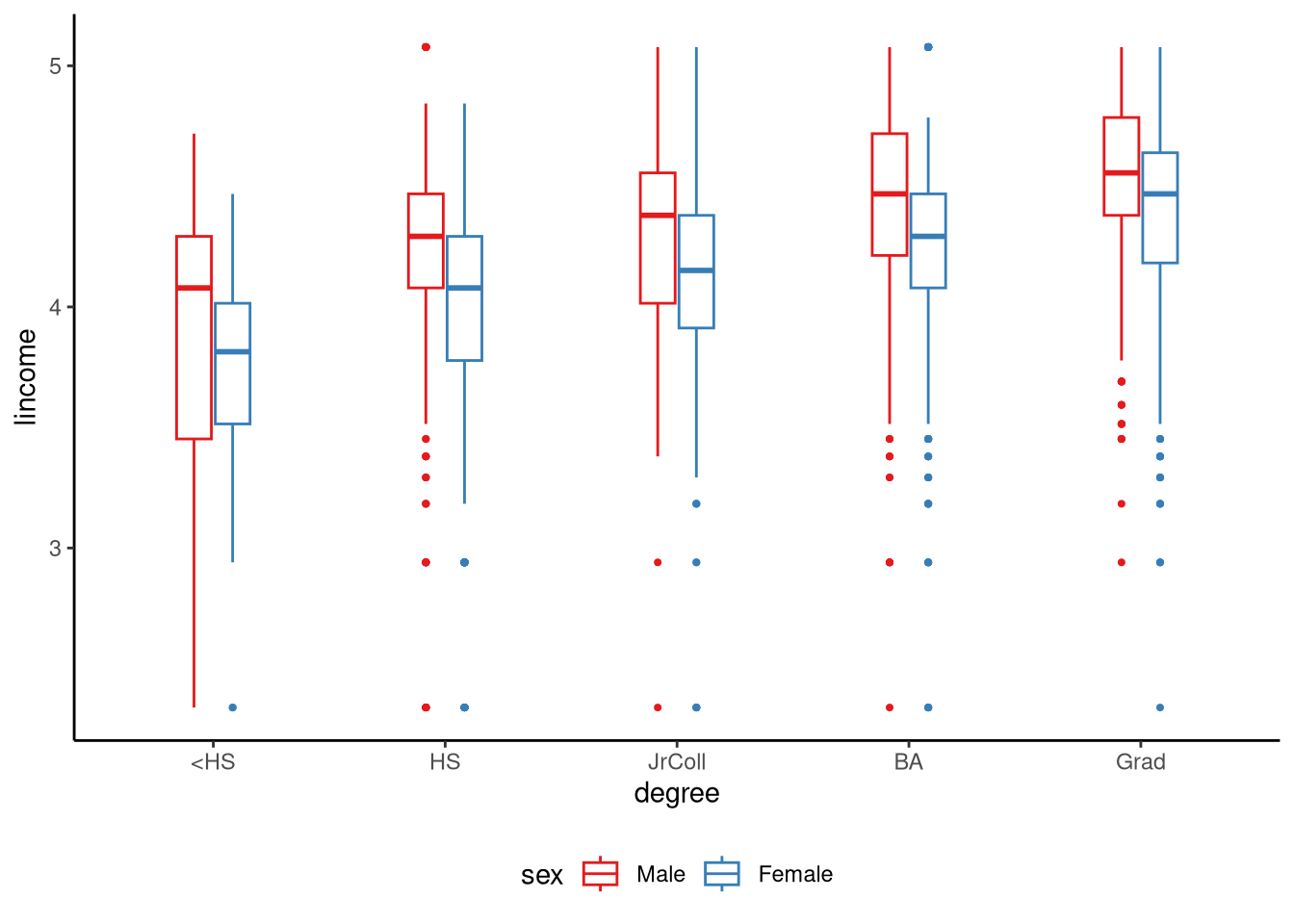
9.3.1 Statistical model
In a two-way ANOVA model, we have two factors (categorical predictors). Let the first factor have \(J\) levels and the second factor have \(K\) levels. We write \(y_{jki}\) for the \(i\)-th observation taken at the combination of level \(j\) of the first factor and level \(k\) of the second factor. Indices therefore range as \(j=1,\dots ,J\), \(k=1,\dots ,K\), and \(i=1,\dots ,n_{jk}\) where \(n_{jk}\) is the sample size in cell (factor combination) \((j,k)\).
The simplest two-factor model assumes that the two factors influence the outcome in an additive fashion. More precisely, the additive model says that every measurement \(y_{jki}\) taken at level \(j\) of the first factor and level \(k\) of the second factor comes from a normal distribution whose mean is the simple sum of two separate contributions. This can be written as \[ y_{jki}\sim N(\mu_{j}+\nu_{k},\sigma^{2}). \] The term \(\mu_{j}\) represents how far the \(j\)-th level of the first factor shifts the outcome variable on average, and the term \(\nu_{k}\) does the same for the \(k\)-th level of the second factor. Because the model is additive these two shifts are combined by addition, so the expected value for a particular cell \((j,k)\) is \(\mu_{j}+\nu_{k}\). Every cell shares the same spread \(\sigma^{2}\), meaning that the natural variability of the outcome is assumed equal across all combinations of the two factors. This is the usual homogeneity of variance that we commonly encounter in normal linear, and related, models.
An equivalent and often more convenient parameterisation of this additive model is \[ y_{jki}= \theta+\alpha_{j}+\beta_{k}+\varepsilon_{jki},\qquad \varepsilon_{jki}\sim N(0,\sigma^{2}). \] Here \(\theta\) is the grand or overall mean that would be observed if we averaged over every combination of the two factors. The quantity \(\alpha_{j}=\mu_{j}-\theta\) measures how far the mean for level \(j\) of the first factor sits above or below the grand mean. Likewise \(\beta_{k}= \nu_{k}-\theta\) measures the deviation of level \(k\) of the second factor from that same grand mean. Because the model is additive, the difference created by changing from level \(j_{1}\) to level \(j_{2}\) of the first factor is the same no matter which level of the second factor is present and vice versa.
In practice, the assumption of strict additivity is often too simplistic, because the effect of one factor can depend on the level of another. To allow the effect of one factor to depend on the level of the other (see Note 9.2) we add an interaction term and write \[ y_{jki}= \theta+\alpha_{j}+\beta_{k}+\gamma_{jk}+\varepsilon_{jki},\qquad \varepsilon_{jki}\sim N(0,\sigma^{2}). \] The new parameter \(\gamma_{jk}\) is the extra deviation observed in cell \((j,k)\) beyond what would be predicted by simply adding \(\alpha_{j}\) and \(\beta_{k}\). In other words, it measures how much the effect of one factor changes depending on the level of the other: the hallmark of an interaction. Parameter constraints \(\sum_{j}\alpha_{j}=0\), \(\sum_{k}\beta_{k}=0\), \(\sum_{j}\gamma_{jk}=0\) for every \(k\), and \(\sum_{k}\gamma_{jk}=0\) for every \(j\) keep the model identifiable. These constraints ensure that each parameter represents a unique contribution rather than overlapping with the overall mean or other effects. Setting every \(\gamma_{jk}\) to zero collapses the interaction model back to the additive model, meaning the influence of one factor is independent of the other.
Note 9.2: What is an interaction?
An interaction arises when the influence of one factor on the outcome is not the same at every level of a second factor. In an additive model, we predict a cell mean by adding the average shift produced by factor A to the average shift produced by factor B, so changing factor A from level \(j_{1}\) to level \(j_{2}\) moves every cell by the same amount no matter which level of factor B is present. When an interaction is present that equal shift rule breaks down and the size, or even the direction, of the difference between levels \(j_{1}\) and \(j_{2}\) depends on which level of factor B we are looking at.
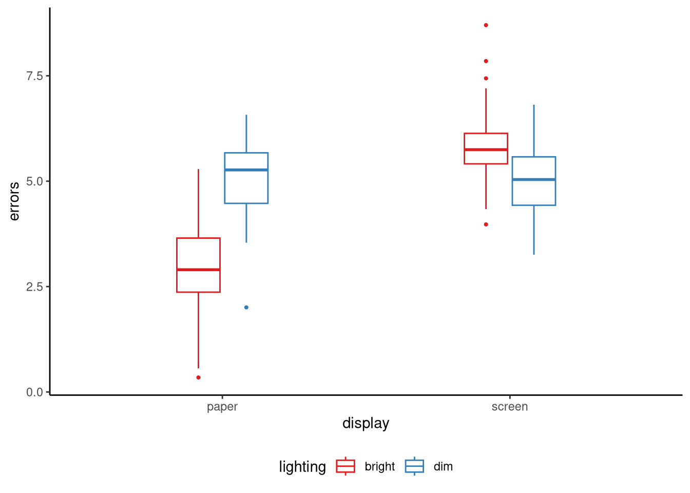
A simple example uses two categorical factors in a study of proofreading accuracy. Factor A is display format with two levels, paper and screen, and factor B is ambient lighting with two levels, bright and dim. If the mean error rate drops by the same amount when we move from screen to paper in both lighting conditions the two factors combine additively. If the drop is large under bright light but vanishes, or perhaps reverses, under dim light the size of the format effect has changed across the lighting levels and we say the factors interact. See Figure 9.3 for an illustration of this scenario.
Total variation is measured by the sum of squares \[ V=\sum_{j=1}^{J}\sum_{k=1}^{K}\sum_{i=1}^{n_{jk}}(y_{jki}-\bar y)^{2}, \] where \(\bar y\) is the grand sample mean. The total variation \(V\) is just the variance of all the observations multiplied by \(n-1\), where \(n=\sum_{j=1}^J\sum_{k=1}^K n_{jk}\) is the total number of observations across all combinations of factors.
Two-way ANOVA partitions this total into four orthogonal, or non-overlappig, pieces (see Note 9.3): \[ V = V_{\alpha}+V_{\beta}+V_{\gamma}+V_{\epsilon}. \]
- \(V_\alpha\) is the variability among the marginal means of the first factor. This is the variation attributable to differences between the levels of the first factor.
- \(V_\beta\) is the variability among the marginal means of the second factor, or variation attributable to differences between the levels of the second factor.
- \(V_\gamma\) is the variability among cell means that remains after the two main effects have been removed. It represents the extra variation produced when the influence of one factor changes across the levels of the other factor.
- \(V_\epsilon\) is the residual variation left after all systematic effects have been accounted for.
Note 9.3: Variance partition in two-way ANOVA
The two-way ANOVA partitions the total sum of squares \[ V = \sum_{j=1}^{J}\sum_{k=1}^{K}\sum_{i=1}^{n_{jk}}(y_{jki}-\bar y)^{2} \] into four non-overlapping pieces \[ V = V_{\alpha}+V_{\beta}+V_{\gamma}+V_{\epsilon}. \]
The term \[ V_{\alpha}= \sum_{j=1}^{J} n_{j\cdot}\,(\bar y_{j\cdot}-\bar y)^{2} \] captures variation explained by the first factor, where \(n_{j\cdot}=\sum_{k} n_{jk}\) and \(\bar y_{j\cdot}\) is the mean across all observations that share level \(j\). The term \[ V_{\beta}= \sum_{k=1}^{K} n_{\cdot k}\,(\bar y_{\cdot k}-\bar y)^{2} \] captures variation explained by the second factor, where \(n_{\cdot k}=\sum_{j} n_{jk}\) and \(\bar y_{\cdot k}\) is the mean for level \(k\). The interaction sum of squares \[ V_{\gamma}= \sum_{j=1}^{J}\sum_{k=1}^{K} n_{jk}\,(\bar y_{jk}-\bar y_{j\cdot}-\bar y_{\cdot k}+\bar y)^{2} \] measures how far each cell mean \(\bar y_{jk}\) departs from what would be predicted by the additive model. The residual term \[ V_{\epsilon}= \sum_{j=1}^{J}\sum_{k=1}^{K}\sum_{i=1}^{n_{jk}}(y_{jki}-\bar y_{jk})^{2} \] records the unexplained within-cell variation.
The corresponding degrees of freedom are \(\text{df}_{\alpha}=J-1\), \(\text{df}_{\beta}=K-1\), \(\text{df}_{\gamma}=(J-1)(K-1)\), and \(\text{df}_{\epsilon}=n-JK\) where \(n=\sum_{j}\sum_{k} n_{jk}\). Dividing each sum of squares by its degrees of freedom forms the mean squares: \[ M_{\alpha} = \frac{V_\alpha}{J-1},\quad M_{\beta} = \frac{V_\beta}{K-1},\quad M_{\gamma} = \frac{V_\gamma}{(J-1)(K-1)},\quad M_{\epsilon} = \frac{V_\epsilon}{n-JK}. \]
9.3.2 Testing main effects and interactions
In a two-way ANOVA the statistical model is \(y_{jki}= \theta+\alpha_{j}+\beta_{k}+\gamma_{jk}+\varepsilon_{jki}\) where \(\theta\) is the grand mean, \(\alpha_{j}\) is the deviation associated with level \(j\) of the first factor, \(\beta_{k}\) is the deviation associated with level \(k\) of the second factor, and \(\gamma_{jk}\) is the extra departure found in cell \((j,k)\) beyond the sum of the two main effects. This formulation leads to three separate null hypotheses, each assessed with its own F test.
The main-effect test for the first factor is of the null hypothesis \[ H_{0}^{A}:\alpha_{1}=\alpha_{2}= \dots =\alpha_{J}=0. \] In other words, this null states that if we gather together all observations that share the same level \(j\) of the first factor, averaging over every level of the second factor, the mean response is the same for every one of the \(J\) levels.
The main-effect test for the second factor is of the the null hypothesis \[ H_{0}^{B}:\beta_{1}= \beta_{2}= \dots =\beta_{K}=0. \] Here the idea is analogous: if we pool all observations that share each level \(k\) of the second factor, ignoring which level of the first factor they belong to, the average response should be identical for all \(K\) levels under the null.
The interaction test compares the full model with a reduced additive model and uses the null hypothesis \[ H_{0}^{AB}:\gamma_{1,1}= \ldots = \gamma_{jk}= \ldots \gamma_{JK}=0 \] for every combination of \(j\) and \(k\). This hypothesis says that once we add together the separate deviations \(\alpha_{j}\) and \(\beta_{k}\) we can perfectly predict each cell mean, so the two factors act independently. The effect of one factor is the same no matter which level of the other factor is present.
The hypotheses just stated are all tested with F tests, each of which requires us to calculate an F statistic that has an F distribution when the null hypothesis is true. An F statistic in ANOVA is built by comparing two nested regression models (see Section 8.7): a reduced or baseline model and a full model. The reduced model omits the term whose effect we want to test. We fit both models, take their residual sums of squares \(\text{RSS}_{\text{reduced}}\) and \(\text{RSS}_{\text{full}}\), subtract them to find the extra variation the term explains, and use this difference as a crucial ingredient in the calculation of the F statistic.
We have different choices about which model counts as the baseline and which model counts as the full model. Statistical software therefore offers three major conventions, usually called Type I, Type II, and Type III sums of squares. In a so-called balanced design, which is where every combination of factors has the same sample size, these three types of calculations all lead to identical results. In addition, Type II and III always lead to the same F statistic for the interaction hypothesis test. However, for unbalanced analyses, which are the common scenario in non-experimental settings, these three ways of formulating the F tests can lead to important distinctions with respect to the main effects, and so understanding the difference between them is of practical importance.
To understand the differences between Type I, II, and III sums of squares, it is helpful to examine the specific model comparisons that each approach uses when testing effects. Consider a two-way ANOVA model with factors A and B, plus their interaction A:B, specified as ~ A + B + A:B.
- Type I sums of squares
-
This follows a sequential approach where the order of terms in the model matters. When testing the main effect of A, Type I compares an intercept-only model (
~ 1) against a model containing only factor A (~ A). For the main effect ofB, it compares the model~ Aagainst the model~ A + B. Finally, for the interaction effect, Type I compares~ A + Bagainst the full model~ A + B + A:B. This sequential testing means that each effect is evaluated after accounting for all effects that appear earlier in the model formula. - Type II sums of squares
-
This tests each main effect while controlling for the other main effect, but not for the interaction. When testing the main effect of
A, Type II compares~ Bagainst~ A + B, effectively asking whetherAadds anything beyond whatBalready explains. Similarly, for the main effect ofB, it compares~ Aagainst~ A + B. The interaction test remains the same as in Type I, comparing~ A + Bagainst~ A + B + A:B. - Type III Sums of Squares
-
This tests each effect in the presence of all other effects in the model. For the main effect of
A, Type III compares~ B + A:Bagainst the full model~ A + B + A:B, asking whether A contributes anything even whenBand theA:Binteraction are already in the model. For the main effect ofB, it compares~ A + A:Bagainst~ A + B + A:B. The interaction test remains~ A + Bversus~ A + B + A:B, identical to Type II. This approach tests the unique contribution of each effect after accounting for all other effects.
The debate over the relative merits of these three approaches can get quite arcane. Following the recommendation of Langsrud (2003a), we will use Type II as our default.
9.3.3 Using aov()
As we did with one-way ANOVA, we can conduct a two-way ANOVA using aov:
M_9_4 <- aov(lincome ~ degree * sex, data = gss2021)The formula syntax here is lincome ~ degree * sex. The * operator is used for factorial analysis: main effects and the interaction of the terms. Writing degree * sex is in fact equivalent to degree + sex + degree:sex, which more explicitly states the main effects and interaction. Thus, an identical model to M_9_4 is M_9_5:
M_9_5 <- aov(lincome ~ degree + sex + degree:sex, data = gss2021)As mentioned, there are three ways of conducting the F test to test the main effects and interaction. Each of these can be obtained from the tidy_anova_ssq() function from sgsur. By default, following our general advice here, this function defaults to Type II:
tidy_anova_ssq(M_9_4) # type = 'II' by default# A tibble: 4 × 5
term sumsq df statistic p.value
<chr> <dbl> <dbl> <dbl> <dbl>
1 degree 62.4 4 71.9 1.17e-57
2 sex 26.9 1 124. 4.51e-28
3 degree:sex 0.582 4 0.670 6.13e- 1
4 Residuals 528. 2434 NA NA The first three rows provide the F statistics and p-values for each of three F tests. We can write each F test result as follows:
- Main effect of
degree: F(4, 2434) = 71.92, p < 0.001 - Main effect of
sex: F(1, 2434) = 123.74, p < 0.001 - Interaction effect: F(4, 2434) = 0.67, p = 0.613
From this, we can see that there are main effects of both degree and sex. In other words, after controlling for the effects of degree, there is still a significant difference in average lincome for the different levels of the sex variable. Likewise, after controlling for the effects of sex, there is still a significant difference in average lincome for the different levels of the degree variable. To be clear, these interpretations are based on the definition of main effect F tests in a Type II sums of squares analysis. The effect of sex is determined by comparing a full model ~ sex + degree and a reduced model ~ degree. The effect of degree is determined by comparing a full model ~ sex + degree and a reduced model ~ sex.
There is no significant interaction effect. This tells us that the full model with the interaction term, ~ sex + degree + sex:degree, is not significantly different to the additive model ~ sex + degree. In other words, the effect of level of education on average income is not different for men and women. Or conversely, the difference between the average incomes of men and women does not differ for the different levels of education.
9.3.4 Follow-up comparisons
Just as we did with the one-way ANOVA (see Section 9.1.3), we can conduct pairwise t-test based comparisons. This may be done in different ways, but the most straightforward in terms of interpretation is to compare all pairs of levels of one factor separately for each level of the other factor. For example, in the following, separately for males and females, we perform all pairwise comparisons of the levels of education:
emmeans(M_9_4, specs = pairwise ~ degree | sex)$emmeans
sex = Male:
degree emmean SE df lower.CL upper.CL
<HS 3.86 0.0811 2434 3.70 4.02
HS 4.22 0.0227 2434 4.17 4.26
JrColl 4.27 0.0464 2434 4.18 4.36
BA 4.41 0.0251 2434 4.36 4.46
Grad 4.53 0.0293 2434 4.48 4.59
sex = Female:
degree emmean SE df lower.CL upper.CL
<HS 3.70 0.0702 2434 3.57 3.84
HS 3.97 0.0218 2434 3.93 4.01
JrColl 4.05 0.0383 2434 3.98 4.13
BA 4.23 0.0243 2434 4.18 4.28
Grad 4.34 0.0281 2434 4.29 4.40
Confidence level used: 0.95
$contrasts
sex = Male:
contrast estimate SE df t.ratio p.value
<HS - HS -0.3615 0.0842 2434 -4.292 0.0002
<HS - JrColl -0.4122 0.0934 2434 -4.412 0.0001
<HS - BA -0.5571 0.0849 2434 -6.563 <0.0001
<HS - Grad -0.6786 0.0862 2434 -7.870 <0.0001
HS - JrColl -0.0507 0.0516 2434 -0.982 0.8635
HS - BA -0.1957 0.0338 2434 -5.783 <0.0001
HS - Grad -0.3171 0.0371 2434 -8.558 <0.0001
JrColl - BA -0.1450 0.0527 2434 -2.751 0.0472
JrColl - Grad -0.2665 0.0548 2434 -4.859 <0.0001
BA - Grad -0.1215 0.0386 2434 -3.150 0.0143
sex = Female:
contrast estimate SE df t.ratio p.value
<HS - HS -0.2659 0.0735 2434 -3.615 0.0028
<HS - JrColl -0.3505 0.0800 2434 -4.382 0.0001
<HS - BA -0.5288 0.0743 2434 -7.116 <0.0001
<HS - Grad -0.6404 0.0756 2434 -8.466 <0.0001
HS - JrColl -0.0846 0.0441 2434 -1.921 0.3065
HS - BA -0.2630 0.0326 2434 -8.055 <0.0001
HS - Grad -0.3745 0.0356 2434 -10.528 <0.0001
JrColl - BA -0.1783 0.0453 2434 -3.932 0.0008
JrColl - Grad -0.2898 0.0475 2434 -6.103 <0.0001
BA - Grad -0.1115 0.0371 2434 -3.003 0.0226
P value adjustment: tukey method for comparing a family of 5 estimates For each set of pairwise comparisons (those corresponding to sex = Male or sex = Female), the procedure is just like that followed in the case of the one-way ANOVA. An adjustment is applied to the p-values to control the FWER (see Note 9.1), which defaults to Tukey’s HSD method.
Given the absence of an interaction effect, the pairwise comparisons of education levels performed separately for males and females should largely match one another. In addition, they should match the pairwise comparisons of education levels averaged across males and females, which is the analysis performed in the one-way ANOVA aov(lincome ~ degree) above.
An alternative analysis is to compare males and females for each education level:
emmeans(M_9_4, specs = pairwise ~ sex | degree)$emmeans
degree = <HS:
sex emmean SE df lower.CL upper.CL
Male 3.86 0.0811 2434 3.70 4.02
Female 3.70 0.0702 2434 3.57 3.84
degree = HS:
sex emmean SE df lower.CL upper.CL
Male 4.22 0.0227 2434 4.17 4.26
Female 3.97 0.0218 2434 3.93 4.01
degree = JrColl:
sex emmean SE df lower.CL upper.CL
Male 4.27 0.0464 2434 4.18 4.36
Female 4.05 0.0383 2434 3.98 4.13
degree = BA:
sex emmean SE df lower.CL upper.CL
Male 4.41 0.0251 2434 4.36 4.46
Female 4.23 0.0243 2434 4.18 4.28
degree = Grad:
sex emmean SE df lower.CL upper.CL
Male 4.53 0.0293 2434 4.48 4.59
Female 4.34 0.0281 2434 4.29 4.40
Confidence level used: 0.95
$contrasts
degree = <HS:
contrast estimate SE df t.ratio p.value
Male - Female 0.153 0.1070 2434 1.427 0.1537
degree = HS:
contrast estimate SE df t.ratio p.value
Male - Female 0.249 0.0315 2434 7.899 <0.0001
degree = JrColl:
contrast estimate SE df t.ratio p.value
Male - Female 0.215 0.0601 2434 3.571 0.0004
degree = BA:
contrast estimate SE df t.ratio p.value
Male - Female 0.181 0.0349 2434 5.196 <0.0001
degree = Grad:
contrast estimate SE df t.ratio p.value
Male - Female 0.191 0.0406 2434 4.715 <0.0001Here, no p-value adjustments are necessary because for each level of education, there is only one pair being compared. Again, given the absence of the interaction, the differences in average income between males and females should be largely the same for each level of education. Likewise, these differences should match those obtained from a standard t-test, t.test(lincome ~ sex), which effectively averages across each level of education when comparing males and females.
9.3.5 Factorial ANOVA as a general linear model
The two-way ANOVA just performed is a type of general linear model. We can perform this exactly as we did with aov() in M_9_4 by using lm() instead:
M_9_6 <- lm(lincome ~ degree * sex, data = gss2021)To verify that this is the same as model M_9_4, we can look at the ANOVA table produced by tidy_anova_ssq() for M_9_6:
tidy_anova_ssq(M_9_6)# A tibble: 4 × 5
term sumsq df statistic p.value
<chr> <dbl> <dbl> <dbl> <dbl>
1 degree 62.4 4 71.9 1.17e-57
2 sex 26.9 1 124. 4.51e-28
3 degree:sex 0.582 4 0.670 6.13e- 1
4 Residuals 528. 2434 NA NA This is identical to that produced using M_9_4:
all.equal(tidy_anova_ssq(M_9_4), tidy_anova_ssq(M_9_6))[1] TRUEUnder the surface in lm(), R converts the two categorical predictor variables to dummy variables in the manner we described previously in Section 9.2.1. We can use get_dummy_code() to see the dummy variables and coding for used for sex and degree as follows:
get_dummy_code(gss2021, sex)# A tibble: 2 × 2
sex sexFemale
<fct> <dbl>
1 Male 0
2 Female 1get_dummy_code(gss2021, degree)# A tibble: 5 × 5
degree degreeHS degreeJrColl degreeBA degreeGrad
<fct> <dbl> <dbl> <dbl> <dbl>
1 <HS 0 0 0 0
2 HS 1 0 0 0
3 JrColl 0 1 0 0
4 BA 0 0 1 0
5 Grad 0 0 0 1In addition, there are dummy variables to represent the interaction terms. We can see the dummy codes for the two factors and their interaction as follows:
get_dummy_code(gss2021, degree * sex)# A tibble: 10 × 11
degree sex degreeHS degreeJrColl degreeBA degreeGrad sexFemale
<fct> <fct> <dbl> <dbl> <dbl> <dbl> <dbl>
1 <HS Male 0 0 0 0 0
2 <HS Female 0 0 0 0 1
3 HS Male 1 0 0 0 0
4 HS Female 1 0 0 0 1
5 JrColl Male 0 1 0 0 0
6 JrColl Female 0 1 0 0 1
7 BA Male 0 0 1 0 0
8 BA Female 0 0 1 0 1
9 Grad Male 0 0 0 1 0
10 Grad Female 0 0 0 1 1
# ℹ 4 more variables: `degreeHS:sexFemale` <dbl>,
# `degreeJrColl:sexFemale` <dbl>, `degreeBA:sexFemale` <dbl>,
# `degreeGrad:sexFemale` <dbl>We can focus on the interaction terms by selecting columns as follows:
get_dummy_code(gss2021, degree * sex) |>
  select(degree:sex, contains(':'))
# A tibble: 10 × 6
degree sex `degreeHS:sexFemale` `degreeJrColl:sexFemale` `degreeBA:sexFemale` `degreeGrad:sexFemale`
<fct> <fct> <dbl> <dbl> <dbl> <dbl>
1 <HS Male 0 0 0 0
2 <HS Female 0 0 0 0
3 HS Male 0 0 0 0
4 HS Female 1 0 0 0
5 JrColl Male 0 0 0 0
6 JrColl Female 0 1 0 0
7 BA Male 0 0 0 0
8 BA Female 0 0 1 0
9 Grad Male 0 0 0 0
10 Grad Female 0 0 0 1These interaction dummy codes are obtained by multiplying the dummy code for each value of sex by that of each value of degree.
This demonstrates a fundamental insight: factorial ANOVA, even with complex interaction effects, is simply multiple linear regression with categorical predictors represented by dummy codes, which we refer to as the general linear model. The model lincome ~ degree * sex is mathematically equivalent to a linear regression with 9 predictor variables (4 for degree, 1 for sex, and 4 for their interactions) plus an intercept. The ANOVA framework provides a convenient way to organise, test, and interpret these effects, but underneath it all, we’re still fitting the linear model:
\[ \begin{split} \text{lincome} = \beta_0 &+ (\beta_1\times\text{degreeHS}) + (\beta_2\times\text{degreeJrColl}) + (\beta_3\times\text{degreeBA}) + (\beta_4\times\text{degreeGrad}) \\ & +\, (\beta_5\times\text{sexFemale}) + (\beta_6\times\text{degreeHS:sexFemale}) \\ & +\, (\beta_7\times\text{degreeJrColl:sexFemale}) + (\beta_8\times\text{degreeBA:sexFemale})\\ & +\, (\beta_9\times\text{degreeGrad:sexFemale}) + \epsilon \end{split} \]
Whether we call it factorial ANOVA or a general linear model is simply a matter of perspective and emphasis — the underlying statistical machinery is identical.
9.4 Mixing categorical and continuous variables
Given that categorical predictors can be used in lm(), we can mix categorical and continuous predictor variables, including with interactions. As an example, in the following model, average log income is modelled as a linear function of a continuous variable, age, and a categorical predictor degree:
M_9_7 <- lm(lincome ~ degree + age, data = gss2021)When a regression model incorporates at least one categorical predictor and at least one continuous predictor, the resulting model structure creates what is known as a varying intercept model. This type of model represents a sophisticated analytical framework that allows for both group differences and relationships with continuous variables to be modelled simultaneously.
To understand the mathematical structure of varying intercept models, consider the simple case where we have one binary categorical predictor and one continuous predictor. In this scenario, the mean of the outcome variable can be expressed as:
\[ \mu = \beta_0 + \beta_1 x + \beta_2 z, \]
where \(x\) represents the continuous variable and \(z\) represents the dummy variable coding for the binary categorical predictor.
The dummy variable \(z\) takes values of either 0 or 1 exclusively, which creates two distinct linear relationships.
- When \(z = 0\) (representing the reference category), the mean becomes a linear function of \(x\): \[ \mu = \beta_0 + \beta_1 x. \]
- When \(z = 1\) (representing the non-reference category), the mean becomes a different linear function of \(x\): \[ \mu = (\beta_0 + \beta_2) + \beta_1 x. \]
This mathematical structure reveals why these models are called “varying intercept” models. The two groups have different intercepts (\(\beta_0\) versus \(\beta_0 + \beta_2\)) but share the same slope (\(\beta_1\)) with respect to the continuous predictor. This assumption implies that the relationship between the continuous predictor and the outcome variable has the same strength and direction in both groups, but the groups differ in their baseline levels.
We can look at the results using a typical ANOVA table:
tidy_anova_ssq(M_9_7)# A tibble: 3 × 5
term sumsq df statistic p.value
<chr> <dbl> <dbl> <dbl> <dbl>
1 degree 62.0 4 67.9 1.92e-54
2 age 3.03 1 13.3 2.72e- 4
3 Residuals 533. 2337 NA NA What is shown here is effectively two model comparisons, just like those described in Section 8.7 and in Section 9.3.2. Both are described by F-tests.
- The effect of
degree: F(4, 2337) = 67.91, p < 0.001. This tests the null hypothesis that knowing a person’s level of education, once we know their age, tells us nothing about their average income. - The effect of
age: F(1, 2337) = 13.29, p < 0.001. This tests the null hypothesis that knowing a person’s age, once we know their level of education, tells us nothing about their average income.
We can also look at the results from the point of view of typical multiple regression analysis. For example, we can use tidy() to view the coefficients table:
tidy(M_9_7, conf.int = TRUE)# A tibble: 6 × 7
term estimate std.error statistic p.value conf.low conf.high
<chr> <dbl> <dbl> <dbl> <dbl> <dbl> <dbl>
1 (Intercept) 3.66 0.0637 57.4 0 3.53 3.78
2 degreeHS 0.305 0.0579 5.26 1.57e- 7 0.191 0.418
3 degreeJrColl 0.362 0.0636 5.69 1.43e- 8 0.237 0.487
4 degreeBA 0.547 0.0584 9.36 1.77e-20 0.433 0.662
5 degreeGrad 0.654 0.0595 11.0 2.04e-27 0.537 0.770
6 age 0.00243 0.000667 3.65 2.72e- 4 0.00112 0.00374We can interpret this table by first concentrating on the age row. Here, 0.00243 is the estimate of the slope coefficient for age: the change in log income for a one unit (one year) change in age. We know, both from the p-value in the coefficient table and the ANOVA table results above, that the null hypothesis for this coefficient can be rejected. The confidence interval is 0.00112, 0.00374.
For the degree variable, the base or reference level is <HS, which corresponds to the value of the intercept coefficient 3.66. This tells us that when degree = <HS, the linear equation is \[
\text{average log income} = 3.66 + 0.00243 \times \text{age}.
\] The remaining coefficients for the degree variable are the differences between the intercept corresponding to degree = <HS and each of the other levels. For example, when degree = HS, the intercept increases by 0.305 so that the linear equation is \[
\begin{aligned}
\text{average log income} &= 3.66 + 0.00243 \times \text{age},\\
&= (3.66 + 0.305) + 0.00243 \times \text{age},
\end{aligned}
\]
We can use emmeans() to look at the predicted average log income for each age from 20 to 60 in increments of 10 years for each education level:
age_seq <- seq(20, 60, by = 10)
emmeans(M_9_7, specs = ~ age | degree, at = list(age=age_seq))
degree = <HS:
age emmean SE df lower.CL upper.CL
20 3.71 0.0584 2337 3.59 3.82
30 3.73 0.0567 2337 3.62 3.84
40 3.75 0.0557 2337 3.65 3.86
50 3.78 0.0556 2337 3.67 3.89
60 3.80 0.0562 2337 3.69 3.91
degree = HS:
age emmean SE df lower.CL upper.CL
20 4.01 0.0251 2337 3.96 4.06
30 4.03 0.0205 2337 3.99 4.08
40 4.06 0.0174 2337 4.03 4.09
50 4.08 0.0165 2337 4.05 4.12
60 4.11 0.0182 2337 4.07 4.14
degree = JrColl:
age emmean SE df lower.CL upper.CL
20 4.07 0.0358 2337 4.00 4.14
30 4.09 0.0330 2337 4.03 4.16
40 4.12 0.0314 2337 4.05 4.18
50 4.14 0.0311 2337 4.08 4.20
60 4.17 0.0322 2337 4.10 4.23
degree = BA:
age emmean SE df lower.CL upper.CL
20 4.25 0.0254 2337 4.20 4.30
30 4.28 0.0213 2337 4.24 4.32
40 4.30 0.0187 2337 4.27 4.34
50 4.33 0.0184 2337 4.29 4.36
60 4.35 0.0204 2337 4.31 4.39
degree = Grad:
age emmean SE df lower.CL upper.CL
20 4.36 0.0292 2337 4.30 4.42
30 4.38 0.0251 2337 4.33 4.43
40 4.41 0.0223 2337 4.36 4.45
50 4.43 0.0213 2337 4.39 4.47
60 4.46 0.0223 2337 4.41 4.50
Confidence level used: 0.95 Here, we are using emmeans() to calculate the predicted average log income for every combination of age in age_seq and level of education, which we could also have done using augment() (see, for example, Section 7.5 and Section 8.9) or other tools.
9.5 Further reading
Øyvind Langsrud’s “ANOVA for unbalanced data: Use Type II instead of Type III sums of squares” (Langsrud, 2003b) explains why Type II sums of squares are generally preferable for unbalanced designs, showing how the choice reflects different model comparisons.
Maxwell and Delaney’s Designing Experiments and Analyzing Data (Maxwell et al., 2017) provides comprehensive coverage of factorial ANOVA, interactions, and contrasts with detailed worked examples from psychological research.
9.6 Chapter summary
- ANOVA is mathematically equivalent to linear regression with categorical predictors, representing a special case of the general linear model rather than a distinct statistical method.
- One-way ANOVA partitions total variance into between-group and within-group components, using the F-statistic to test whether group means differ more than expected by chance alone.
- Dummy coding converts categorical predictors into numeric variables, with coefficients representing group differences relative to a chosen reference level whose selection affects coefficient values but not model fit or F-tests.
- The F-test in one-way ANOVA compares a model with group means to an intercept-only model, testing the omnibus hypothesis that all group means are equal in the population.
- Pairwise comparisons examine specific group differences using estimated marginal means, with adjustments like Tukey HSD controlling family-wise error rate when conducting multiple tests simultaneously.
- Factorial ANOVA includes multiple categorical predictors and their interactions, allowing the effect of one factor to vary across levels of another factor.
- Interaction effects indicate that the relationship between one predictor and the outcome depends on the value of another predictor, requiring conditional interpretation of main effects when interactions are present.
- Type I, Type II, and Type III sums of squares differ in how they partition variance when predictors are correlated, with Type II generally preferred for unbalanced designs because it tests meaningful marginal hypotheses.
- ANCOVA combines categorical and continuous predictors in the same model, estimating group differences while statistically controlling for continuous covariates.
- Understanding ANOVA as regression with categorical predictors unifies analysis of group comparisons and continuous relationships under the general linear model framework, preparing for repeated-measures and mixed-effects extensions.