df_heart_angina <- heartdisease |>
  mutate(heart_disease_prob = ifelse(heart_disease == "yes", 1, 0)) |>
filter(angina == 'yes')12 Logistic regression
In all the chapters so far, we have assumed that the outcome variable being modelled is continuous and, at least in principle, ranges from negative infinity to infinity. For these outcome variables, we assumed that each observation was drawn from a normal distribution in the population and that they can be modelled using the general linear model. However, not all of our outcome variables will be continuous. Sometimes we want to model data that represent binary, categorical, ordinal, or count outcomes. Let us recall what these data types are:
Binary: Binary data represent variables that can only take one of two mutually exclusive categories. Example: the outcome of a pregnancy test (positive/negative)
Categorical: Categorical data represent variables that have mutually exclusive values, but these values do not have any natural ordering (i.e., one group is not higher/better/larger than any other). Binary data is a special case of categorical data. Example: diet preference (omnivore, vegetarian, vegan).
Ordinal: Ordinal data are similar to categorical data in that they represent variables with mutually exclusive values. However, in contrast to categorical variables, ordinal variables do have a natural ordering. Example: highest level of education (primary school < secondary school < university).
Count: Count data represent the number of times something happened. They must have values that are non-negative integers. Example: the number of mouse clicks an individual makes on a website
When modelling data of these types, assuming that the outcome variable is modelled by a normal distribution is no longer possible, and we need to utilise new models that allow us to replace the normal distribution with something more appropriate. For these cases, we can use a generalisation of the general linear model known as the generalised linear model.
The chapter covers
- Generalised linear models extend regression to non-normal outcomes by combining a probability distribution, link function, and linear predictor.
- Binary logistic regression models probabilities using the logit link that transforms probabilities to log-odds, ensuring predictions stay between 0 and 1.
- Coefficients in logistic regression represent changes in log-odds, which can be exponentiated to odds ratios for more intuitive interpretation.
- Multinomial logistic regression extends binary models to unordered categorical outcomes with more than two levels by comparing each category to a reference.
- Ordinal logistic regression models ordered outcomes using proportional odds, treating them as arising from an underlying continuous latent variable.
- Model evaluation uses deviance statistics and likelihood ratio tests to compare nested models and assess whether predictors improve fit.
12.1 The generalised linear model
The generalised linear model is, in many ways, very similar to the general linear model. In fact, we can think of this model as just an extension of the general linear model, rather than something completely new. Recall the definition of the general linear model. We have observed data that can be written as follows: \[ (y_1, \vec{x}_1), (y_2, \vec{x}_2) \ldots (y_n, \vec{x}_n), \] where \(y_1, y_2 \ldots y_n\) are the observed values of the outcome variable, and for each one, we have a vector of \(K\) predictor or explanatory variables \(\vec{x}_i\), i.e., \(\vec{x}_i = [x_{1i}, x_{2i} \ldots x_{Ki}]^\intercal\). We then assume the following statistical model of the \(y_1, y_2 \ldots y_n\): \[ \begin{aligned} y_i &\sim N(\mu_i, \sigma^2),\quad\text{for $i \in 1, 2 \ldots n$},\\ \mu_i &= \beta_0 + \sum_{k=1}^K \beta_k x_{ki}. \end{aligned} \] This model has two main components:
- A probabilistic family that specifies how each observation of the outcome variable \(y_i\) is distributed in the population — here, normally distributed with mean \(\mu_i\) and standard deviation \(\sigma\).
- A deterministic component that describes how \(\mu_i\) varies as a linear function of the \(K\) predictors at observation \(i\), \(x_{1i}, x_{2i}, \ldots, x_{Ki}\).
Although this form is sufficient for the general linear model, it is helpful to express it in a more general way that will make the next step — the generalised linear model — easier to understand. We can write the linear model as: \[ \begin{aligned} y_i &\sim N(\mu_i, \sigma^2),\quad\text{for $i \in 1, 2 \ldots n$},\\ g(\mu_i) &= \phi_i,\quad \phi_i = \beta_0 + \sum_{k=1}^K \beta_k x_{ki}. \end{aligned} \] Here we have introduced a link function \(g(\cdot)\), which connects the parameter of the probabilistic component (the mean, \(\mu_i\)) to the linear predictor \(\phi_i\), see Note 12.1. The link function simply defines how the expected value of the outcome relates to the predictors. In the general linear model, this link is the identity function, meaning that \(g(\mu_i) = \mu_i\) — the mean of the outcome is directly modelled as a linear function of the predictors. In general, it is a smooth and invertible function — meaning that it changes gradually (no jumps or breaks) and allows us to move back and forth between the scale of the outcome and the scale of the predictors, as we’ll see in the examples later in this chapter. Because this identity link leaves values unchanged (for any \(x\), \(g(x) = x\)), it is not usually written explicitly. Writing it this way, however, helps us see how the general linear model can be viewed as one member of a much broader family of models.
The generalised linear model (GLM) extends this idea by allowing both different outcome distributions and different link functions. Instead of assuming normality, we let the outcome follow a probability distribution \(P(\cdot)\) appropriate to its type.
It can be written as: \[ \begin{aligned} y_i &\sim P(\theta_i, \psi),\quad\text{for $i \in 1, 2 \ldots n$},\\ g(\theta_i) &= \phi_i,\quad \phi_i = \beta_0 + \sum_{k=1}^K \beta_k x_{ki}, \end{aligned} \] where \(P(.)\), as we will see, is some probability distribution whose main parameter is \(\theta_i\), and which might also have some optional nuisance parameters, which we denote by \(\psi\). Then, we have some link function \(g(\cdot)\), such that the link function of the main parameter \(\theta_i\) is a linear function of the vector of predictor variables \(\vec{x}_i\).
Using different probability distributions and different link functions gives us different types of generalised linear models. We will begin with arguably the most widely used type of generalised linear model, namely the binary logistic regression model.
Note 12.1: Understanding link functions
A link function tells the model how to connect two worlds: the world of the outcome variable (which so far has been continuous, but could also represent probabilities, categories, or counts) and the world of the predictors (which, in a linear model, combine in a straight-line or additive way).
In the general linear model, this connection is simple — we use the identity link, so the mean of the outcome is itself a linear function of the predictors.
For other outcome types, however, the link must transform the outcome’s scale so that it can be modelled linearly. For example: - In logistic regression, the link turns probabilities (0–1) into log-odds. - In Poisson regression, the link turns counts (0, 1, 2, …) into their logarithm. Both log-odds and logarithms theoretical range from \(-\infty\) to \(\infty\), allowing us to model them with a straight-line relationship.
In other words, think of the link as a translator. Probabilities, counts, or categories can’t be modelled directly with a straight line — they live on restricted scales. The link function converts those values into something linear, lets us fit the model, and then converts them back so we can interpret results in the original units. This ability to move back and forth between scales is what we mean when we say a link function is invertible.
12.2 Binary logistic regression
Binary logistic regression is used when we have an outcome variable that is binary and so has only two mutually exclusive values. The values of binary variables could be, for example, right handed/left handed, correct/incorrect, yes/no, etc. No matter what these values are, we can formally represent these values simply by \(0\) and \(1\). As such, we say that each observed value of the outcome variable \(y_i\) always takes the value of either \(0\) or \(1\) only.
For modelling binary outcome data, we cannot use a general linear model, which assumes that each value of \(y_i\) has been drawn from a normal distribution. We’ll use a dataset which is concerned with health and demographic information for 270 patients who were admitted to hospital with chest pain and were later found to have heart disease or not. In this example, our predictors will be whether the individual had exercise induced angina (where \(1\) means Yes, and \(0\) means No) and their resting blood pressure (measured in mm Hg) when they were admitted to the hospital. The outcome variable will be heart disease, which has values of yes or no. Ultimately, we are interested in how the probability of having heart disease changes as a function of our predictors, angina and resting blood pressure. Let us try modelling this data using a general linear model and see the shortcomings of that approach.
Let us say we are trying to predict the probability of someone having heart disease based on their resting blood pressure but we are only interested in individuals who have angina. We convert the binary variable to 0s and 1s to represent the probability of being in each group:
In our general linear model, we estimate coefficients that describe a linear relationship between the mean of the outcome variable and the predictor. However, it is difficult to see how a linear relationship, or straight line, would best capture the relationship between a binary outcome and a continuous predictor. A further complication is that our outcome variable is bounded at \(0\) and at \(1\). That means that if we did use a general linear model to model these data, the predictions we make from our model would need to be constrained to be between 0 and 1.
M_12_1 <- lm(heart_disease_prob ~ resting_bp, data = df_heart_angina)
summary(M_12_1)$coefficients
Estimate Std. Error t value Pr(>|t|)
(Intercept) 0.289081692 0.292957262 0.9867709 0.3262100
resting_bp 0.003589735 0.002174331 1.6509605 0.1019808From this, our intercept term is saying that when resting_bp is 0, the average of the heart disease variable is 0.289. The slope term is saying that for every one unit increase in resting_bp, the average of the heart disease variable increases by 0.004. So far, this is not meaningless. However, let us see what happens when we try to predict the average of the heart disease variable when a person’s resting_bp is 200: \[
0.289 + 0.004 \times 200 = 1.007.
\] The prediction is greater than 1. This is meaningless because the average of the values of a binary variable can only range from \(0\) to \(1\). Additionally, binary outcome data violate the normality assumption of linear regression since the residuals from such models cannot be normally distributed.
Instead of modelling \(y_1, y_2 \ldots y_n\) using a linear model, we need to use some suitable generalised linear model. To do this, we make a number of changes to the normal linear model. First, we must treat each \(y_i\) as having been drawn from a probability distribution that can only take values of \(0\) and \(1\). There is, in fact, only one possible probability distribution to choose from here, and that is the Bernoulli distribution. Unlike the normal distribution, which is described by two parameters, usually denoted by \(\mu\) and \(\sigma\), the Bernoulli distribution has just one parameter, which is usually denoted by \(\theta\) (theta). The \(\theta\) parameter tells us the probability that \(y_i\) takes the value of \(1\). In other words, if \(y_i\) is described by a Bernoulli distribution, then \[ \mathrm{P}\!\left(y_i = 1\right) \triangleq \theta. \] where the symbol \(\triangleq\) means “is defined as”.
Because \(y_i\) has only two values, we therefore know that \[ \mathrm{P}\!\left(y_i = 0\right) = 1- \theta. \] As an example, imagine we have a binary variable that represents handedness and so takes on the values of left and right, which we can represent by \(0\) and \(1\), respectively. If the probability of being right handed is 90%, then \(\theta = 0.9\), and the probability of being left-handed is \(1-\theta = 0.1\).
Now that we know that the Bernoulli distribution best describes our binary variable, we can use this as the probabilistic component in our generalised linear model instead of the normal distribution. Thus far, our statistical model of \(y_1, y_2 \ldots y_n\) is as follows: \[ y_i \sim \textrm{Bernoulli}(\theta_i),\quad \text{for $i \in 1, 2 \ldots n$}. \] This means that each value of the outcome variable is assumed to be sampled from a Bernoulli distribution instead of a normal distribution. For each \(y_i\), the corresponding value of the Bernoulli parameter is \(\theta_i\).
In a general linear model, we assumed that the mean of the main parameter of the outcome variable varies as a linear function of the predictors. When using a Bernoulli distribution, we cannot have each \(\theta_i\) varying as a linear function of the predictors. The reason for this is because each \(\theta_i\) can only have values between \(0\) and \(1\). In order to deal with this constraint, we choose a link function \(g(\cdot)\) that transforms \(\theta\) so that it can have values from \(-\infty\) to \(\infty\). Although there are many options of suitable link functions to choose from, the canonical and default choice for the binary logistic regression is the logit function, which has the following form: \[ g(\theta) = \textrm{logit}(\theta) = \ln\left(\frac{\theta}{1 - \theta}\right). \] In the last term, we see that we first need to divide \(\theta\) by \(1- \theta\). Dividing \(\theta\) by \(1- \theta\) takes our probabilities and turns them into odds. You might be familiar with odds if you have ever placed a bet, but put simply, they represent the chance of something happening divided by the chance of that thing not happening. We then calculate the natural logarithm of the odds to get the log odds. The log odds is also known as the \(\textrm{logit}\) function, see @#nte-probs-odds-logodds.
Note 12.2: Probability, odds, and log-odds
Understanding how probabilities are transformed in logistic regression helps make sense of the logit link.
- Probability (\(\theta\))
- The proportion of times an event occurs, bounded between 0 and 1. Example: if a student passes an exam 8 times out of 10, the probability of passing is 0.8.
- Odds (\(\theta / (1 - \theta)\))
- The ratio of the chance an event happens to the chance it does not. Using the same example, the odds of passing are \(0.8 / (1 - 0.8) = 4\), meaning “four to one.”
- Log-odds (\(\ln(\theta / (1 - \theta))\))
- The natural logarithm of the odds. Log-odds transform the bounded probability scale (0–1) into an unbounded scale (\(-\infty\) to \(\infty\)), which allows us to model them linearly with predictors. Log-odds are sometimes called the logit. They are less intuitive than probabilities but make the mathematics of logistic regression possible. You can always convert them back to probabilities after fitting the model.
Having specified that the probabilistic component is a Bernoulli distribution, and that the link function is a logit function, what about the deterministic component? We can still assume that the deterministic component of the model is the same as in the general linear model, i.e., a linear function.
The full statistical model is, therefore, as follows: \[ \begin{aligned} y_i &\sim \textrm{Bernoulli}(\theta_i),\quad\text{for $i \in 1, 2 \ldots n$},\\ g(\theta_i) &= \ln\left(\frac{\theta}{1 - \theta}\right) = \phi_i,\quad \phi_i = \beta_0 + \sum_{k=1}^K \beta_k x_{ki}. \end{aligned} \] Writing this more compactly, we have \[ \begin{aligned} y_i &\sim \textrm{Bernoulli}(\theta_i),\quad\text{for $i \in 1, 2 \ldots n$},\\ \ln\left(\frac{\theta}{1 - \theta}\right) &= \beta_0 + \sum_{k=1}^K \beta_k x_{ki}. \end{aligned} \]
Here we are saying that each observation of the outcome variable \(y_i\) is drawn from a Bernoulli distribution in the population. For each observation, the Bernoulli distribution is specified by one parameter, \(\theta_i\), which represents the probability that the outcome takes the value of \(1\) and not \(0\). Since \(\theta_i\) is bounded between \(0\) and \(1\), we use the logit link function to transform \(\theta_i\) into log odds, which is unbounded, and treat the log odds as a linear function of the predictors.
What we will do now is work through an example of binary logistic regression. Showing how the model works practically should help clarify some of the above.
12.2.1 Binary logistic regression in R
To see binary logistic regression in action we’ll use the volunteering dataset from the sgsur package, which details the personality traits of individuals who do and do not volunteer to take part in psychological research:
volunteering# A tibble: 1,421 × 4
neuroticism extraversion sex volunteer
<int> <int> <fct> <fct>
1 16 13 female no
2 8 14 male no
3 5 16 male no
4 8 20 female no
5 9 19 male no
6 6 15 male no
7 8 10 female no
8 12 11 male no
9 15 16 male no
10 18 7 male no
# ℹ 1,411 more rowsThe dataset has 1421 observations and four variables. We will focus on two variables:
volunteer- This has levels yes and no. This is our outcome variable.
extraversion- This details an individual’s extraversion score calculated from the Eysenck personality inventory (Eysenck & Eysenck (1963)). Scores range from 0 to 24, with higher scores representing higher levels of extraversion.
Let’s visualise the variables together using a boxplot, see Figure 12.1.
tukeyboxplot(y = extraversion, x = volunteer, data = volunteering)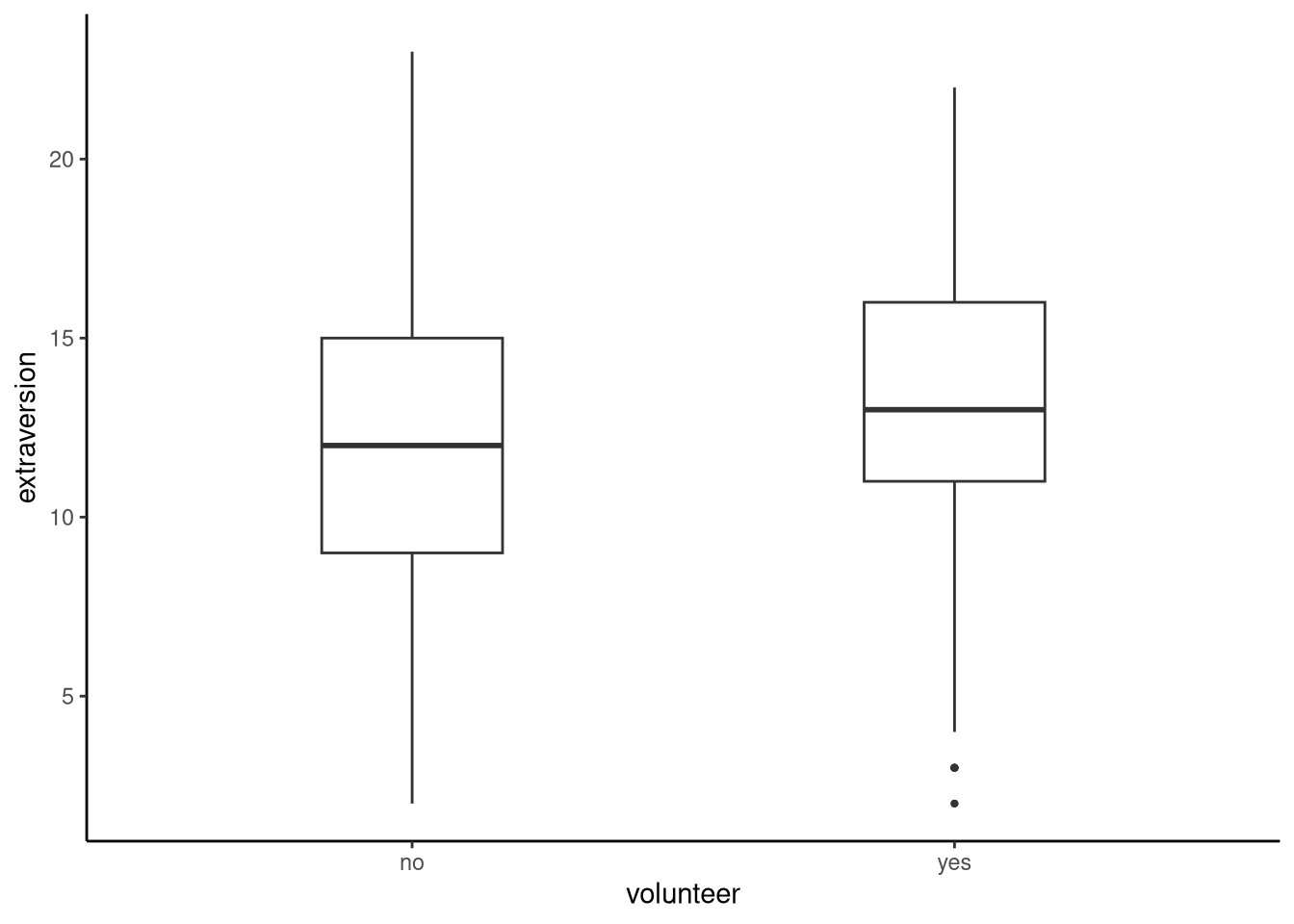
Looking at this plot we can see that the mean levels of extraversion are slightly higher in those who volunteer than those who do not. For our model, we will see if extraversion predicts whether an individual volunteers for psychological research or not (volunteer). As such, our outcome variable will be volunteer, a binary variable, and our predictor will be extraversion, a continuous variable. Remember that in binary logistic regression we use the Bernoulli distribution which is specified by one parameter, \(\theta\), which represents the probability that the outcome variable will take on one of the levels of the binary variable. Because of this, R will choose one level of our binary variable to model by default. Sometimes this default is meaningful for our data, other times we may want to change this. Either way, it is important that we check which level the default is so that we can understand the outputs of our model; we can do this using contrasts.
pull(volunteering, volunteer) |>
  contrasts()
yes
no 0
yes 1This output shows us which level of the outcome variable R has chosen as a default to represent \(\theta\). Since the 1 is against the row with yes we conclude that \(\theta\) will represent an observation recording yes in the variable volunteer, in other words, our model will predict the probability of an individual being a volunteer:
M_12_2 <- glm(volunteer ~ extraversion,
                   data = volunteering,
                   family = binomial(link = "logit"))
This code is very similar to the lm() code we used to run our linear regressions in previous chapters, with a couple of changes. First, note that we use glm() to denote that we want to use a generalised linear model. We also specify the type, or family, of generalised linear model. Here we want to run a binary logistic model which we specify using binomial. Finally, we specify the link function, which here is logit. Let’s take a look at the output:
summary(M_12_2)
Call:
glm(formula = volunteer ~ extraversion, family = binomial(link = "logit"),
    data = volunteering)

Coefficients:
             Estimate Std. Error z value Pr(>|z|)
(Intercept)  -1.13942    0.18538  -6.146 7.93e-10 ***
extraversion  0.06561    0.01414   4.640 3.49e-06 ***
---
Signif. codes:  0 '***' 0.001 '**' 0.01 '*' 0.05 '.' 0.1 ' ' 1

(Dispersion parameter for binomial family taken to be 1)

    Null deviance: 1933.5  on 1420  degrees of freedom
Residual deviance: 1911.5  on 1419  degrees of freedom
AIC: 1915.5

Number of Fisher Scoring iterations: 4
First, let’s look at the coefficients directly:
coef(M_12_2) (Intercept) extraversion
-1.13941868 0.06561304 To make sense of these, it often helps to translate between the three related scales used in logistic regression: log-odds, odds, and probabilities. The intercept of -1.1394 represents the log-odds of volunteering when extraversion = 0. Converting this with the inverse logit function, plogis(-1.139), gives a probability of about 24%. This means that when extraversion is 0, the model predicts a 24% chance of volunteering.
The slope of 0.0656 tells us that each one-point increase in extraversion raises the log-odds of volunteering by that amount. Exponentiating this with exp(0.066) ≈ 1.07 shows that the odds of volunteering increase by about 7% for each point of extraversion. Because the logit scale is non-linear, this does not mean the probability rises by a constant amount — effects are larger around 0.5 and smaller near the extremes.
To see how this relationship looks across the full range of extraversion, we can calculate the model’s predicted probabilities directly.
newdata <- tibble(extraversion = seq(0, 24, by = 1))

volunteer_predictions <- newdata |>
  mutate(predicted_volunteer = predict(M_12_2,
                                       newdata = newdata),
         predicted_volunteer_probs = plogis(predicted_volunteer))

volunteer_predictions
# A tibble: 25 × 3
extraversion predicted_volunteer predicted_volunteer_probs
<dbl> <dbl> <dbl>
1 0 -1.14 0.242
2 1 -1.07 0.255
3 2 -1.01 0.267
4 3 -0.943 0.280
5 4 -0.877 0.294
6 5 -0.811 0.308
7 6 -0.746 0.322
8 7 -0.680 0.336
9 8 -0.615 0.351
10 9 -0.549 0.366
# ℹ 15 more rowsThe first column of predictions gives the log-odds from the model, and the second column shows the same values converted into probabilities using the inverse logit function plogis(). This allows us to interpret and visualise the model’s results on the familiar 0–1 probability scale.
These predictions are shown in Figure 12.2.
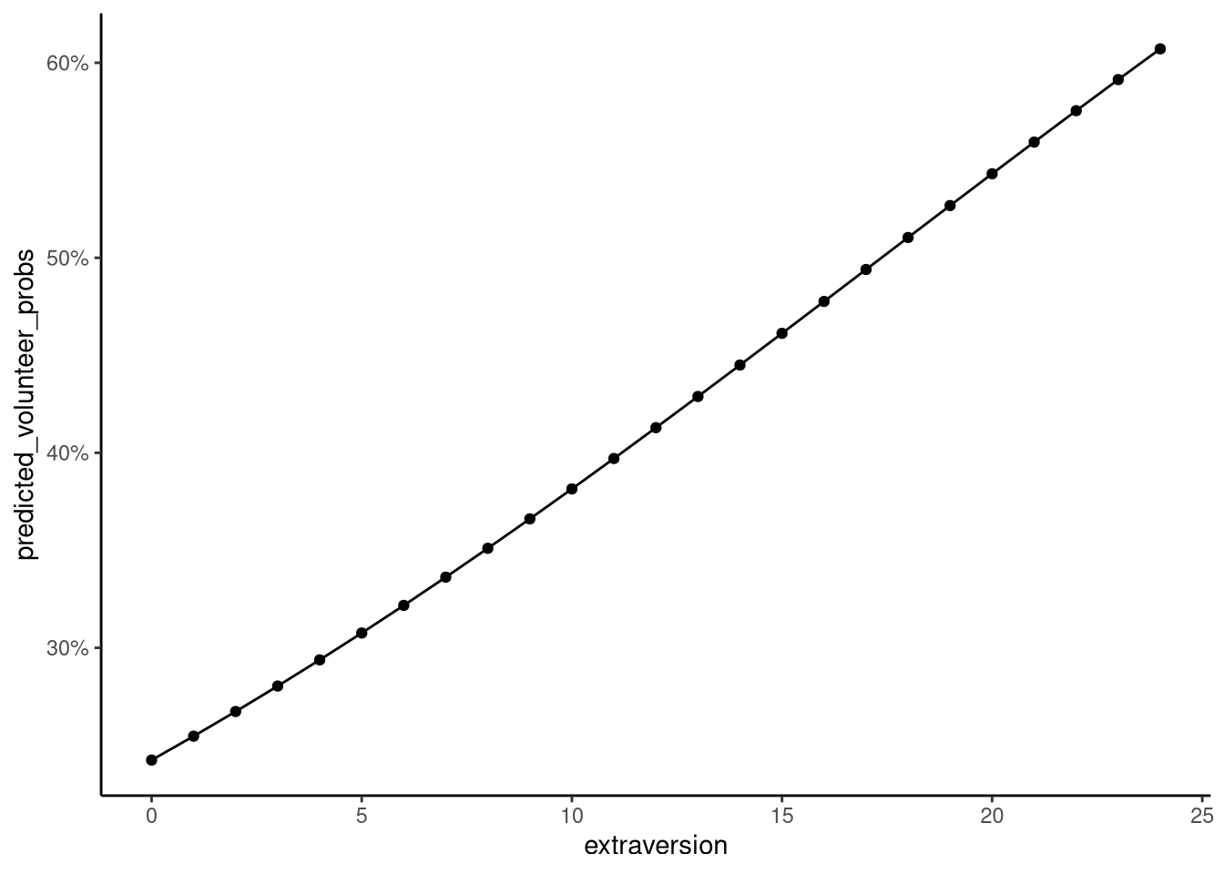
From this plot, we can see a clear increase in the probability of volunteering as extraversion rises. The probability passes 50% only once extraversion scores reach around 17, and even at the highest score of 24, the predicted chance of volunteering is only about 60%. Visualising model predictions in this way helps turn abstract coefficients into something interpretable, revealing how predicted probabilities change across the range of extraversion.
Now that we have an idea of the relationship between extraversion and the probability of volunteering, let’s take a look at the hypothesis tests associated with our model:
summary(M_12_2)$coefficients Estimate Std. Error z value Pr(>|z|)
(Intercept) -1.13941868 0.18538042 -6.146381 7.927081e-10
extraversion 0.06561304 0.01414193 4.639609 3.490697e-06The standard error represents the standard deviation of the sampling distribution of each estimate. If we were to repeatedly draw samples from the population, the estimates would vary slightly each time; the standard error tells us how much. Smaller values indicate that the estimates are more stable across samples. In a linear model, we typically test coefficients using the t-statistic, because the residual variance must be estimated. In logistic regression, however, there is no separate variance term. Because of this, and because the maximum-likelihood estimates are (asymptotically) normally distributed, we use the z-statistic instead. It’s conceptually the same ratio — estimate divided by its standard error — but compared against the standard normal distribution rather than t.
Note 12.3: Why z instead of t in logistic regression?
Both t- and z-statistics test whether a coefficient differs from zero, but they arise from slightly different assumptions about how we estimate uncertainty.
In a linear model, we estimate both the coefficients and the residual variance (\(\sigma^2\)). Because (\(\sigma^2\)) is unknown and must be estimated from the data, the resulting sampling distribution of the coefficients has extra uncertainty. That’s why we use the t-statistic: \[ t = \frac{\hat{\beta}}{\text{SE}(\hat{\beta})} \] which follows a t-distribution with \(n - k\) degrees of freedom.
In a GLM, the outcome distribution itself, for example, a Bernoulli distribution for binary data, defines the variance as a function of the mean.
\[ \text{Var}(Y_i) = \theta_i(1 - \theta_i) \] This variance is largest when \(\theta_i = 0.5\) (the outcome is most uncertain) and smallest when \(\theta_i\) is near 0 or 1 (the outcome is almost fixed). Because the variance is already specified by the distribution, there is no separate residual variance to estimate.
Because the variance is already specified by the distribution, there is no separate residual variance to estimate. Under fairly general conditions, the estimates are asymptotically normal — meaning that as the sample size \(n\) grows large, the sampling distribution of each estimated coefficient approaches a normal (bell-shaped) distribution, centred on the true value. \[ \hat{\beta} \sim N(\beta, \text{Var}(\hat{\beta})) \]
This property allows us to use the standard normal distribution, and therefore z-statistics, rather than t-statistics, because the model does not require estimating a separate residual variance.
We can also easily obtain the 95% confidence intervals for the estimates using:
confint(M_12_2) 2.5 % 97.5 %
(Intercept) -1.50604145 -0.77891167
extraversion 0.03804996 0.09351843The confidence interval gives us the set of hypothetical values of the coefficients that are compatible with the data. For example, any hypothetical value of the slope coefficient between around 0.04 and 0.09 is not incompatible with the data.
Finally, the output of our model provides two measures of model fit: the null deviance and the residual deviance. Put simply, the null deviance measures how well a model with no predictors fits the data, whereas the residual deviance measures how well the model fits after including our predictors. Both are based on the log-likelihood of the model — a measure of how probable the observed data are under the fitted parameters.
Formally, the deviance is defined as \[ D = -2 \left[ \ell_{\text{model}} - \ell_{\text{saturated}} \right], \] where \(\ell_{\text{model}}\) is the log-likelihood of our fitted model, and \(\ell_{\text{saturated}}\) is the log-likelihood of a saturated model (one that fits the data perfectly). Smaller deviance values therefore indicate a model whose predicted probabilities are closer to the observed outcomes.
The null deviance uses the log-likelihood of a model with only an intercept (no predictors), \[ D_0 = -2 \left[ \ell_{\text{null}} - \ell_{\text{saturated}} \right], \] and the residual deviance uses the log-likelihood from the model with our predictor(s), \[ D_1 = -2 \left[ \ell_{\text{model}} - \ell_{\text{saturated}} \right]. \] The difference between the two, \[ \Delta D = D_0 - D_1, \] tells us how much the inclusion of predictors improves model fit. Under large-sample conditions, this difference approximately follows a \(\chi^2\) distribution with degrees of freedom equal to the number of predictors added.
We can illustrate this comparison explicitly by fitting a model with no predictors and then comparing it to our extraversion model. If you look closely at the output, you’ll see that the difference in deviance matches what is reported in the model summary. In our case, the predictor extraversion reduces the deviance, meaning the model with extraversion fits the data significantly better than the model with no predictors.
M_12_3 <- glm(volunteer ~ 1,
                   data = volunteering,
family = binomial(link = "logit"))anova(M_12_3, M_12_2, test = 'Chisq')Analysis of Deviance Table
Model 1: volunteer ~ 1
Model 2: volunteer ~ extraversion
Resid. Df Resid. Dev Df Deviance Pr(>Chi)
1 1420 1933.5
2 1419 1911.5 1 22.022 2.695e-06 ***
---
Signif. codes: 0 '***' 0.001 '**' 0.01 '*' 0.05 '.' 0.1 ' ' 112.3 Categorical Logistic Regression
So far, we have explored a model that allows us to examine binary categorical variables — those that only have two levels. We can now extend this model to examine categorical variables with more than two levels. This model goes by several names, including multinomial logistic regression and polytomous logistic regression, but we shall refer to it as categorical logistic regression.
In categorical logistic regression, we model an outcome variable that has more than two possible categories. In other words, the outcome values are \(y_1, y_2, \ldots, y_n\), and each \(y_i\) takes one of \(J\) categorically distinct values, which we can represent by \(1, 2, \ldots, J\). Examples of categorical variables with more than two levels might include a student’s programme of study (e.g., Economics, Sociology, Politics, Criminology) or their dietary preference (e.g., omnivore, vegetarian, vegan, pescatarian).
Formally, we assume that each observation is drawn from a categorical distribution: \[ y_i \sim \textrm{Categorical}(\pi_i),\quad\text{for $i \in 1, 2 \ldots n$}. \]
The parameter \((\pi_i)\) (pi) is a vector of probabilities describing the chance that observation \(i\) belongs to each category of the outcome:
\[ \pi_{i} = [\pi_{1i}, \pi_{2i}, \ldots \pi_{Ji}], \] where \[ P(y_i = j) \triangleq \pi_{ji}. \]
For example, if an outcome has three categories and the probabilities for a given observation are [0.25,0.5,0.25], this means there is a 25% chance of category 1, 50% chance of category 2, and 25% chance of category 3.
Note how \(\pi_i\) is a vector, not a single value. This contrasts with binary logistic regression, where each \(\theta_i\) represented one probability (e.g., the probability of “success”), and with general linear models, where each \(\mu_i\) represented one expected value. Because \(\pi_i\) is vector-valued, the link function and deterministic component of the model become more complex.
To describe how these probabilities depend on the predictor variables \(x_{1i}, x_{2i}, \ldots, x_{Ki}\) we model each non-reference category relative to a chosen base category.
In particular, for each \(j \in 2, \ldots, J\), \[ \log\left(\frac{\pi_{ji}}{\pi_{1i}}\right) = \beta_0^j + \sum_{k=1}^K \beta^j_{k} x_{ki} \] This means that the deterministic component consists of \(J-1\) separate linear models. Each one models the log of the probability that \(y_i = j\) compared to the probability that \(y_i = 1\). Here, the first value of the outcome variable is known as the reference, or base, category. It makes no difference which category serves as the reference, but — as in binary logistic regression, we must always specify which one it is.
Let us this description into context. Suppose we are interested in how an individual’s dietary status varies with a set of \(K\) predictors. For simplicity, imagine the outcome has three categories: omnivore (1), vegetarian (2), and vegan (3). In a categorical logistic regression, we arbitrarily choose one category, say omnivore, as the reference category. The model then compares the probability of being in each of the other categories to the probability of being in the reference category. Thus, we estimate two log-odds comparisons: vegetarian versus omnivore, and vegan versus omnivore.
The link and deterministic components for these comparisons are:
\[ \log\!\left(\frac{P(y_i = \text{vegetarian})}{P(y_i = \text{omnivore})}\right) = \log\!\left(\frac{\pi_{2i}}{\pi_{1i}}\right) = \beta_0^{(2)} + \sum_{k=1}^K \beta_k^{(2)} x_{ki}, \] and
\[ \log\!\left(\frac{P(y_i = \text{vegan})}{P(y_i = \text{omnivore})}\right) = \log\!\left(\frac{\pi_{3i}}{\pi_{1i}}\right) = \beta_0^{(3)} + \sum_{k=1}^K \beta_k^{(3)} x_{ki}. \]
Each equation describes how the predictors change the log-odds of being in one dietary category relative to the baseline category of omnivore.
12.3.1 Categorical logistic regression in R
To run and interpret categorical logistic regression in R we’ll use the gap52 dataset from the sgsur package. This dataset provides average life expectancy, per capita GDP, and population by continent in 1952. Here we’ll look at the relationship between life expectancy and continent; specifically, we’ll see if we can predict continent based on life expectancy.
Let’s visualise the relationship between continent and life expectancy:
tukeyboxplot(y = lifeExp, x = continent, data = gap52)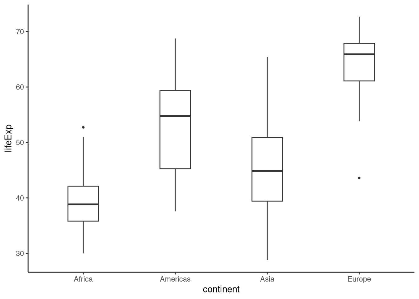
Before we start to run the model, we need to understand which level of the outcome variable R is treating as the reference or baseline. We may also want to change this to make the comparisons in the model more meaningful for our analysis. To understand which level is the baseline, we can use the following code, which should feel familiar from the binary logistic regression above:
gap52 |>
  pull(continent) |>
  contrasts()
Americas Asia Europe
Africa 0 0 0
Americas 1 0 0
Asia 0 1 0
Europe 0 0 1The baseline category is the row which contains only zeroes — or the level which is missing from the columns, for this example that is Africa. Therefore, when we run the model, it will be based on the following comparisons.
- Americas vs Africa
- Asia vs Africa
- Europe vs Africa
If we wanted to change the reference level, we could use the following code; in this example, we set Asia to be the reference:
gap52a <- mutate(gap52, continent = fct_relevel(continent, "Asia"))We can check this using the contrasts function again:
gap52a |>
  pull(continent) |>
  contrasts()
Africa Americas Europe
Asia 0 0 0
Africa 1 0 0
Americas 0 1 0
Europe 0 0 1Here we see Asia now has zeroes in the rows and is missing from the columns and is hence our reference category. We’ll keep this as our reference category in the examples below.
To run categorical regression, we’ll use the multinom() function from sgsur (re-exported from nnet):
M_12_4 <- multinom(continent ~ lifeExp, data = gap52a)The structure of this syntax is identical to our lm() models; we specify our outcome variable continent, our predictor lifeExp and the dataset.
Let’s take a look at the results:
summary(M_12_4)Call:
multinom(formula = continent ~ lifeExp, data = gap52a)
Coefficients:
(Intercept) lifeExp
Africa 6.942099 -0.15376825
Americas -4.394288 0.08274892
Europe -14.617188 0.25682178
Std. Errors:
(Intercept) lifeExp
Africa 1.723294 0.04061513
Americas 1.579758 0.03111592
Europe 3.042951 0.05165635
Residual Deviance: 253.7927
AIC: 265.7927 First, we have our coefficients; we have an intercept and slope term for each of the levels of the categorical variable (excluding the reference level). Remember in our model specification we are modelling the log of the comparison of the probabilities of being in one level of the categorical variable vs the reference level
We’ll convert these to probabilities later to make them easier to interpret, but for now, let’s understand what the coefficients are telling us. For Africa, we see that when life expectancy is zero, the log of the probability ratio of being from Africa compared to being from Asia is 6.942. We see also from the coefficient of the slope that as life expectancy increases by 1 year, the log probability ratio of being from Africa as compared to Asia changes by -0.154. That is, as life expectancy increases, the log probability ratio of being from Africa as compared to Asia reduces.
Next in the model output we have the standard errors — the standard deviation of the sampling distribution. You may also notice that we do not have any t or z statistics, or any corresponding p-values. If these are important to us, we can calculate z statistics and p-values manually as follows:
z <- summary(M_12_4)$coefficients/summary(M_12_4)$standard.errors
pnorm(abs(z), lower.tail=FALSE) * 2
(Intercept) lifeExp
Africa 5.616020e-05 1.531010e-04
Americas 5.408822e-03 7.828561e-03
Europe 1.558203e-06 6.635571e-07Note that we can also get the 95% confidence intervals for the intercept and slope coefficients using confint():
confint(M_12_4), , Africa
2.5 % 97.5 %
(Intercept) 3.5645050 10.31969224
lifeExp -0.2333724 -0.07416406
, , Americas
2.5 % 97.5 %
(Intercept) -7.49055693 -1.298019
lifeExp 0.02176284 0.143735
, , Europe
2.5 % 97.5 %
(Intercept) -20.5812621 -8.6531138
lifeExp 0.1555772 0.3580664As with our other regression models, we are generally interested in the p-value for the slope. As such, the first p-value we are interested in is in the row Africa and the column lifeExp, p < 0.001. This tells us that there is a significant difference in the probability of being from Africa and our reference level, Asia, based on life expectancy. If we were interested in additional comparisons, for example, the Americas vs Europe, we could relevel the outcome variable, making one of these levels the reference level and rerun the model, interpreting the coefficients, z statistics and p-values as appropriate.
Let’s do some predictions based on the model. First, we’ll make some new data, specifying the levels of the predictor we are interested in, say 30 years to around 70 years:
newdata <- tibble(lifeExp = seq(30, 70, by = 1))Our predictions allow us to see the probability of being from each of the continents based on life expectancy:
gap52_pred <- newdata |>
  mutate(predicted_continent = predict(M_12_4, newdata = newdata, type = "prob"))

head(gap52_pred)
# A tibble: 6 × 2
lifeExp predicted_continent[,"Asia"] [,"Africa"] [,"Americas"] [,"Europe"]
<dbl> <dbl> <dbl> <dbl> <dbl>
1 30 0.0876 0.899 0.0129 0.0000872
2 31 0.100 0.883 0.0161 0.000129
3 32 0.115 0.865 0.0200 0.000191
4 33 0.130 0.845 0.0247 0.000281
5 34 0.148 0.821 0.0304 0.000411
6 35 0.167 0.795 0.0373 0.000600 12.4 Ordinal Logistic Regression
As we have seen, categorical logistic regression is used when the outcome variable has multiple categories with no natural ordering. However, when the categories do have a natural order, we need a different model: the ordinal logistic regression.
An example of an ordinal outcome variable is a survey item with responses such as Disagree, Neutral, and Agree. Here the categories follow a clear order — Disagree expresses less agreement than Neutral, which in turn expresses less agreement than Agree. Importantly, this ordering does not imply equal spacing: the difference between Disagree and Neutral may not be the same as the difference between Neutral and Agree.
We can think of such ordinal responses as arising from an underlying, unobserved latent variable that represents the individual’s true level of agreement. This latent variable is assumed to be continuous and follows a logistic distribution, defined by two parameters: a location (its centre) and a scale (its spread). The observed ordinal categories — Disagree, Neutral, and Agree — correspond to thresholds that divide this continuous latent distribution into discrete segments, as shown in Figure 12.4.
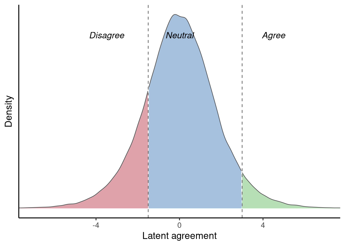
According to this plot, if an individual chose the response option Neutral, their underlying position on the latent agreement scale would fall between roughly −1 and 3. You might wonder what a value like “2” on this scale actually represents. The truth is that the scale itself is arbitrary. In this example, we are trying to capture an individual’s agreement with a statement, but unlike measurable constructs such as height, weight, or response time, there is no physical instrument for “agreement.” Instead, we assume that people have some unobserved, continuous tendency to agree or disagree, and our observed response categories (Disagree, Neutral, Agree) simply reflect intervals on that underlying continuum. The latent variable is therefore a conceptual tool rather than something we can measure directly — its numeric range is arbitrary, but the ordering and cutpoints are meaningful.
To model an ordinal response, we could fit several binary logistic regressions — for example, Disagree vs Neutral, Neutral vs Agree, and Disagree vs Agree. However, this approach treats each comparison as unrelated, ignoring the fact that our response categories are ordered. It also produces multiple, potentially inconsistent estimates for the same predictors.
Instead, we want a single, parsimonious model that respects the ordinal nature of the outcome. Rather than estimating the probability of being in a specific category (as in binary logistic regression), we model the cumulative probability of being in a given category or any category below it on the ordinal scale.
In our three-category example (Disagree, Neutral, Agree), the model estimates:
- the probability of responding Disagree or lower (which is simply Disagree)
- the probability of responding Neutral or lower (that is, Neutral or Disagree)
The probability of being in the highest category (Agree or lower) is always one and is therefore not estimated. Because the highest category is redundant, we fit \(J - 1\) equations — one fewer than the number of response categories.
Using cumulative probabilities allows us to capture the ordinal structure in a single model and to maintain a coherent interpretation of predictor effects.
12.4.1 The proportional odds model
One of the most widely used ordinal logistic models is the proportional odds model. It assumes that the effect of each predictor is constant (or proportional) across all thresholds of the outcome.
Formally, the model can be written as:
\[ \begin{aligned} y_i &\sim \text{Categorical}(\pi_i), \quad \text{for } i = 1, \ldots, n,\\ \text{logit}\big[P(Y_i \le j)\big] &= \zeta_j - \phi_i, \quad \text{with} \quad \phi_i = \beta_0 + \sum_{k=1}^K \beta_k x_{ki}, \quad j = 1, \ldots, J - 1. \end{aligned} \] Where the first line is our probabilistic component, defining how each observation of the outcome variable is distributed in the population — here following a categorical distribution described by cumulative probabilities. The second line is our deterministic component, defining how those cumulative probabilities vary as a linear function of the predictors through the linear predictor \(\phi_i\).
Here:
- \(P(Y_i \le j)\) is the cumulative probability that individual \(i\) is in category \(j\) or below;
- \(\zeta_j\) is the cutpoint (or threshold) on the latent scale separating category \(j\) from \(j + 1\);
- and the linear predictor \(\phi_i\) moves the location of each observation along the latent scale.
Because we assume the latent variable follows a logistic distribution, the link function for these cumulative probabilities is again the logit, just as in binary logistic regression.
12.4.2 Ordinal logistic regression in R
To run an ordinal logistic regression in R we’ll use the depsleep dataset from the sgsur package, which provides data on self-reported depressed mood, usual sleep duration, and employment status for participants aged 18 and over. In this example, we will model the number of days during which the participant felt depressed, recorded as None, Several and Most (more than half the days) against the number of hours sleep the participant usually gets on a given night. Descriptive statistics show that individuals who recorded feeling depressed on None or Several days had similar hours sleep at around 7 hours sleep per night, whereas those who recorded Most had around 6 hours sleep per night.
We’ll use the polr() (proportional odds logistic regression) function from the sgsur package (re-exported from the MASS package) to run our logistic regression. This function uses the same formula that we’ve used for all of our other models so far, such that we need to specify our outcome, predictor and data:
M_12_5 <- MASS::polr(Depressed ~ SleepHrsNight, data = depsleep)Let’s take a look at the output:
summary(M_12_5)Call:
MASS::polr(formula = Depressed ~ SleepHrsNight, data = depsleep)
Coefficients:
Value Std. Error t value
SleepHrsNight -0.2233 0.02315 -9.646
Intercepts:
Value Std. Error t value
None|Several -0.1904 0.1581 -1.2042
Several|Most 1.2393 0.1617 7.6654
Residual Deviance: 8064.669
AIC: 8070.669
(12 observations deleted due to missingness)First, we can see that the model has two parts, the coefficients and the intercepts. The coefficients section is equivalent to our usual regression output, providing us with the log-odds estimate of the slope for the predictor along with the standard error and t-value. We do not get a p-value by default here but can calculate it by comparing the t-value of the slope to the standard normal distribution as follows:
pnorm(abs(summary(M_12_5)$coefficients[1,3]), lower.tail = FALSE) *2[1] 5.124009e-22Our p-value is extremely small, showing us that the probability that we would have obtained this test statistic or one more extreme if the null hypothesis is true is very small. Hence, we can be fairly confident that there is evidence that sleep affects depression scores. Although the p-value is useful for us, we also need to understand what the coefficient is telling us in terms of the size and direction of the effect of sleep on depression scores. The SleepHrsNight coefficient is reported in log-odds. It shows us that a one-hour increase in sleep per night decreases the log-odds of moving into a higher category of the ordinal depression scale (i.e., reporting being more depressed) by -0.2232883. Exponentiating this value, exp(-0.45) \(\approx\) 0.64, shows that each extra hour of sleep multiplies the odds of being in a higher depression category by 0.64 — a 36% reduction in the odds.
Note that we can get the 95% confidence intervals for the slope coefficients using confint():
confint(M_12_5) 2.5 % 97.5 %
-0.2687189 -0.1779633 Next, the model output gives us the estimate of the cutpoints, \(\zeta_1 \text{ and } \zeta_2\). These are the thresholds that divide the latent logistic distribution into the observed response categories. They act like intercepts in that they anchor the cumulative logit equations, but we don’t usually interpret them directly — their specific values depend on how the outcome categories are coded and are mainly used internally to calculate predicted probabilities. In this example, the first cutpoint lies between None and Several and represents the log-odds of responding None or lower when SleepHrsNight is zero. The second cutpoint lies between Several and Most and represents the log-odds of responding Several or lower (that is, Several or None) when SleepHrsNight is zero.
We can make predictions using our model — we’ll create some new data using values of SleepHrsNight that are of interest; let’s use 2-13 as examples. Our predictions allow us to see the probability of choosing each category of Depressed for a given level of SleepHrsNight:
newdata <- tibble(SleepHrsNight = seq(2, 13, by = 1))

#| echo: true
nhanes_predictions <- newdata |>
  mutate(predicted_depressed = predict(M_12_5, newdata = newdata, type = "prob"))

head(nhanes_predictions)
# A tibble: 6 × 2
SleepHrsNight predicted_depressed[,"None"] [,"Several"] [,"Most"]
<dbl> <dbl> <dbl> <dbl>
1 2 0.564 0.280 0.156
2 3 0.618 0.253 0.129
3 4 0.669 0.225 0.106
4 5 0.716 0.197 0.0866
5 6 0.759 0.170 0.0705
6 7 0.798 0.145 0.057212.5 Further reading
Bürkner and Vuorre’s “Ordinal Regression Models in Psychology: A Tutorial” (Bürkner & Vuorre, 2019) provides an accessible introduction to ordinal regression through both frequentist and Bayesian lenses, explaining latent variable thresholds and proportional odds assumptions with practical psychological examples.
Liddell and Kruschke’s “Analyzing Ordinal Data with Metric Models: What Could Possibly Go Wrong?” (Liddell & Kruschke, 2018) demonstrates through simulation how treating ordinal outcomes as continuous can bias estimates and distort inference, advocating for ordinal models that respect the data’s structure.
12.6 Chapter summary
- Generalised linear models (GLMs) extend the normal linear model to non-continuous outcomes by combining a probability distribution appropriate to the outcome type, a link function, and a linear predictor.
- Binary logistic regression models outcomes with two categories using the Bernoulli distribution and the logit link function, which transforms probabilities (bounded 0-1) into log-odds (unbounded).
- Coefficients in binary logistic regression represent changes in log-odds, which can be exponentiated to odds ratios for more intuitive interpretation as multiplicative changes in odds per unit predictor increase.
- Multinomial logistic regression extends binary models to unordered categorical outcomes with more than two levels by comparing each category to a reference category using log-odds ratios.
- Ordinal logistic regression models ordered categorical outcomes using cumulative probabilities and proportional odds, treating categories as thresholds on an underlying continuous latent variable.
- The logit link function transforms probabilities to log-odds by taking the natural logarithm of the odds (probability divided by one minus probability), enabling linear modelling on an unbounded scale.
- Model evaluation uses deviance statistics and likelihood ratio tests to compare nested models, assessing whether adding predictors significantly improves fit beyond what would be expected by chance.
- Predicted probabilities are obtained by applying the inverse logit function (
plogis()inR) to the linear predictor, converting log-odds back to the 0-1 probability scale for interpretation. - The proportional odds assumption in ordinal regression states that predictor effects are constant across all cutpoints, meaning the effect of a predictor does not depend on which threshold is being modelled.
- GLMs unify analysis of diverse outcome types under a common framework of distribution, link function, and linear predictor, with logistic regression preparing the conceptual foundation for count models and other GLM extensions.