urn_sampler(red = 50, black = 50, sample_size = 10) red black
8 2 In every analysis considered in Chapter 3, we were just describing or summarising our data. We did this either by the use of quantitative descriptions and summaries, such as by calculating means and standard deviations, or by the use of visual descriptions and summaries, such as boxplots, histograms, or scatterplots. As important as these descriptive analyses are, they are rarely, if ever, the ultimate objective of our data analyses. Ultimately, our objective is to generalise beyond the specifics of our data. In other words, our objective is not simply to describe or summarise a particular data set. Rather, it is to draw conclusions about a more general phenomenon of which a particular data set is a specific instantiation.
To appreciate how generalisation, rather than the details of a specific data set, is ultimately our objective in statistical analyses, consider a hypothetical study such as the following. We survey 1,000 people in some country and ask them how they will vote in some upcoming election. Let’s say that the electoral candidates in this hypothetical scenario are from political parties named Green, Red, and Blue, and each respondent in the survey just states the candidate that they would most likely vote for. Our data might look something like this: \[ \texttt{red}, \texttt{green}, \texttt{blue}, \texttt{blue}, \texttt{green}, \texttt{red} \ldots \texttt{red}, \texttt{red}, \texttt{green}. \] We could easily summarise this data by stating the proportions of respondents that chose candidates from each of the three parties. From this, we might obtain results like the following: 37.5% of our 1,000 respondents chose a Blue candidate, 23% chose a Green candidate, and 39.5% chose a Red candidate. Were we to conduct a survey like this, however, it is unlikely that we would be interested only in summary statistics like these, which pertain solely to this particular data set. More often, and arguably always, we are ultimately interested in drawing more general conclusions that go beyond the specifics of any one data set. For example, we might be interested in using the results of this survey to draw conclusions about the voting behaviour of all people in the country in the upcoming election. Specifically, we might wish to make statements about the probability that the Red party will receive the most votes, or the majority of the votes, and so on. No amount of descriptions or summaries of the data set itself will be sufficient to allow us to draw these conclusions. To generalise beyond our data, we need statistical inference. This chapter introduces these inferential methods.
It is difficult to overstate the importance of inferential statistics in data analysis. There is arguably no science of statistics without the use of inferential statistics, and virtually every application of statistics in scientific research is based on the use of inferential statistics. Consequently, everything we cover in Part II and Part III in this book will involve inferential statistics.
Despite its importance and ubiquity, however, inferential statistics requires more careful thought than the topics we’ve covered so far. Many of the concepts involve subtle distinctions, and unlike descriptive statistics and visualisation, which often feel intuitive, inferential statistics asks you to think in ways that don’t always align with everyday reasoning. This shift catches many students off guard, and it’s worth noting that even experienced researchers sometimes struggle with these concepts (Greenland et al., 2016; Reinhart, 2015). In fact, academic textbooks occasionally misinterpret fundamental ideas too (Cassidy et al., 2019).
What this means is that you’re likely to find this chapter more challenging than previous ones. Students often notice a gear shift at this point. If you feel that way, you’re in good company. The key is patience and practice. These concepts become clearer with time and repetition, so don’t expect immediate mastery. We recommend proceeding thoughtfully, building understanding step by step, and returning to this chapter as you work through later material.
The chapter covers
Let us begin by outlining a simple problem that will serve as a point of focus for much of the remaining content in this chapter. In 2017, a YouGov survey asked a sample of people between the ages of 16 and 24 in Britain about their use of illegal drugs. This data is available in our sgsur package under the name yougov17drugs. You can learn more about the data and the survey itself by doing ?yougov17drugs and reading the help page.
In total, there were 1,300 respondents, of whom 172 responded that they were currently taking illegal drugs either occasionally or frequently. This is 13.23%. On the basis of this information, assuming that there are no errors in the data and assuming respondents were being truthful, we can state with certainty that 13.23% of the 1,300 respondents were taking illegal drugs at the time of the survey. But can we generalise from these survey results and conclude that 13.23% of all young Britons were current users of illegal drugs at that time?
One reason why we might not be able to generalise from this survey is that the respondents might not be representative of all young people in Britain at the time. For example, perhaps those who responded to the YouGov survey had certain demographic characteristics, or had certain lifestyles or behaviours, that made them more or less likely to take illegal drugs than other young people in Britain. The representativeness of a sample is certainly of great importance when considering whether and how we can generalise from that sample. However, YouGov surveys are designed to be representative of the societies they study (YouGov, 2025), and so we will assume, at least for present purposes, that this survey sample was in fact representative of all young people in Britain in 2017.
Given our assumption that the sample of 1,300 respondents is representative, returning to our main question, can we now say that exactly 13.23% of all young people in Britain were users of illegal drugs in 2017? We cannot, at least not with certainty. The reason for this is sampling variability. Sampling variability means that, in general, any sample of items from a larger group will never perfectly resemble that larger group. Likewise, each sample from the larger group will not perfectly resemble every other sample. What this means for our question is that we cannot know with certainty what the proportion of drug users among all young people in Britain is on the basis of knowing the proportion in our sample. For example, if the true proportion of drug users among all young people in Britain was, say, exactly 10%, then it would not necessarily be the case that exactly 10% of any sample would be drug users. No matter what the true proportion among all young people in Britain is, the proportion in any one sample will not necessarily be identical. Sometimes the proportion in the sample will be higher, sometimes lower, than the true proportion. And so if we find, as we did, that exactly 13.23% of a sample are drug users, then that does not necessarily mean that the proportion among all young people in Britain is 13.23%.
What we have just described is a general problem in all data analysis. Our data, however large, is always only ever a sample from a larger set. In statistical terminology, we call this larger set the population (see Note 4.1). Thus, if we were to do any survey, experiment, or randomised controlled trial, or any other method of data collection, the data from that study would only ever be a sample from a population. Were we to repeat that study, we would obtain yet another sample from the population. We are never interested in just the particular sample. Ultimately, we are always interested in the population from which it was sampled. Because of sampling variability, we cannot know the properties of the population with certainty on the basis of the properties of any sample. Therefore, we must use a body of theoretical results, which we collectively refer to as statistical inference or inferential statistics, to allow us to generalise from any sample to the population.
There are at least two major approaches to statistical inference. One, and the traditionally most widely used approach, is known as classical, or frequentist, or sampling theory-based, inference. The second, which is a more modern approach, and especially useful for more advanced problems, is known as Bayesian inference. Here, we introduce the classical approach to inference, which will be used throughout all chapters in Part II. Later, in Part III, we introduce the Bayesian approach.
In statistics, the term population has a technical meaning that differs from everyday usage. In everyday language, a population is usually the collection of people who live in some region or country. In statistics, on the other hand, a population is the larger group from which our data is a sample, and to which we aim to generalise from our sample. Sometimes this population might be a population of people. But usually the population is not as simple as that, and often is an abstract or hypothetical set.
As an example, imagine that a clinical trial is conducted to test the effectiveness of a new cancer drug. A sample of patients with cancer is used in this trial. The statistical population is the larger set of which these patients are a representative sample. This is not necessarily all cancer patients. It may just be those of a certain age, or with a certain type of cancer, or without certain other ailments. But it is not just the set of currently existing cancer patients with these particular characteristics. It is the set of all possible cancer patients with these characteristics. The population, therefore, is not a finite set of real individuals, but rather a hypothetical set of infinitely many individuals.
Knowing what defines the statistical population is not necessarily obvious. If, for example, we ask all students in some university class to take part in a survey, what is the population of which this set of students is a representative sample? It is not necessarily all people, nor even all university students. After all, these people were students in some particular class in some particular university at some particular time. But likewise, it is not that these students can be seen as representative of no group other than themselves. Were that the case, we could not generalise from this sample to anything. It may never be clear or uncontroversial what the population in this case is, but we can make reasonable judgements about what it is based on our knowledge of the characteristics of the students in this university and those that take particular classes.
In general, whenever we do inferential statistical analysis, we see our data set as a sample from some statistical population. Often, we just have some implicit assumptions about what this population is, but it is always preferable to think more explicitly about this population in order to better appreciate the larger group to which we are generalising.
Although we cannot know the properties of the population with certainty from any single sample, there are systematic relationships between the population and the samples drawn from it. What this means is that sample results are not random in the everyday sense of “completely unpredictable.” Instead, they follow patterns we can describe and quantify.
For example, suppose the true proportion of some variable in the population is 10%. Because of sampling variability, not every sample will show exactly 10%. Some will be higher, some lower. But we can still say which results are more or less likely: obtaining a sample proportion of, say, 5% or 15% is more likely than a sample proportion of 0% or 20%.
In fact, for any possible population proportion, we can work out the probability of obtaining each possible sample proportion. This collection of probabilities is called the sampling distribution.
The sampling distribution is important because it lets us judge whether our observed sample proportion is compatible with a proposed population value. With this, for any given sample proportion, we will be able to effectively rule out, or not rule out, any hypothetical values for the population proportion.
Both sampling variability and sampling distributions are concepts of fundamental importance for understanding statistical inference. In this section, we want to describe and discuss them in more detail. Let us begin with sampling variability. This is quite a simple concept, and can usually be grasped very easily just by seeing some examples of random sampling, which we can easily perform using a programme called urn_sampler from our sgsur R package. Let us imagine we have a jar (statisticians often call this an “urn”, which is just another word for jar) filled with 50 red and 50 black marbles, and let us randomly sample 10 marbles from this jar. Each time we sample a marble, we put it back into the jar. This is known as sampling with replacement. Because there are 50 red and 50 black marbles, the first time we sample, we have a 50% probability of picking a red marble and a 50% probability of picking a black marble. Because we put the marble we picked back into the jar immediately, every time we choose, we have a 50% probability of picking a red marble and a 50% probability of picking a black marble.
To do this urn sampling in R using urn_sampler, we do the following, where we have specified the number of red marbles by red = 50, the number of black marbles with black = 50, and the size of our sample with sample_size = 10:
urn_sampler(red = 50, black = 50, sample_size = 10) red black
8 2 As we can see, in our sample of 10 marbles, we get 8 red ones and 2 black ones. (Note that urn_sampler() uses random sampling, so if you run this same code yourself, you will likely get a different result.) This already tells us a lot. In particular, even though 50% of the marbles in the jar are red and 50% are black, in our sample, 80% of the marbles are red, and 20% are black. Clearly, therefore, the proportions in our sample do not perfectly resemble, and in fact are quite different from, the proportions in the jar. This is exactly a consequence of sampling variability: the properties of a sample will not necessarily match those of the larger set from which the sample was drawn.
Let us now draw another sample of size 10 from the same urn with 50 red and 50 black marbles:
urn_sampler(red = 50, black = 50, sample_size = 10) red black
7 3 Now we get 7 red marbles and 3 black ones, and so in this sample, 70% of the marbles are red, and 30% are black. This is yet another example of sampling variability. Not only do the proportions in this sample not equal those of the jar, but they don’t equal the proportions in the first sample.
But is it the case that every time we draw a sample of size 10 from this jar, we could get any result? In other words, could we get any number of red marbles and any number of black ones on any occasion, or will certain outcomes occur more often? To explore this question, let us do multiple repetitions of this sampling procedure. We can do so in a single urn_sampler command. For example, let us draw 10 samples, each of size 10, from the jar with 50 red and 50 black marbles. To do so, we use the same code as above, but include the argument repetitions = 10 to repeat the sampling process 10 times:
urn_sampler(red = 50, black = 50, sample_size = 10, repetitions = 10)# A tibble: 10 × 2
red black
<int> <int>
1 3 7
2 5 5
3 6 4
4 7 3
5 7 3
6 5 5
7 7 3
8 6 4
9 4 6
10 6 4From this, it seems as if some outcomes are more likely than others. For example, looking at the number of red marbles, we see that we obtained 5 red marbles 2 times, 6 red marbles 3 times, and 7 red marbles 3 times, and so just three numbers of red marbles occur in 8 of the 10 samples.
To get a better sense of whether certain numbers of red and black marbles occur more frequently in samples than other numbers, we can ask urn_sampler to count, or tally, the number of times each unique combination of numbers of red and black marbles occur, and we repeat the sampling process a much larger number of times, specifically 100,000 times, in order to get reliable numbers. To count the number of times each combination of numbers of red and black marbles occur, we use tally = TRUE in urn_sampler. This will return two new columns, tally and prob, which give the frequency and the probability, respectively, of each possible combination of numbers of red and black marbles. The frequency is just the number of times the outcome occurred. The probability, by contrast, in this case, is just the relative frequency, or the frequency divided by the total number of samples.
urn_sampler(red = 50, black = 50, sample_size = 10, repetitions = 100000,
            tally = TRUE)
# A tibble: 11 × 4
red black tally prob
<int> <int> <int> <dbl>
1 0 10 88 0.00088
2 1 9 983 0.00983
3 2 8 4395 0.0440
4 3 7 11810 0.118
5 4 6 20750 0.208
6 5 5 24656 0.247
7 6 4 20244 0.202
8 7 3 11640 0.116
9 8 2 4385 0.0438
10 9 1 955 0.00955
11 10 0 94 0.00094The probabilities in this output are shown in Figure 4.1. As we can see from the output and the figure, every combination of numbers of red and black marbles occur, but do not occur equally often. For example, the most common outcome is 5 red and 5 black marbles. This occurs 24,656 times out of 100,000, which is approximately 24.7% of the time. By contrast, outcomes like 0 red and 10 black marbles occur only 88 times out of 100,000, which is approximately 0.088% of the time, or less than 1 in 1,000 times. Likewise, the outcome of 10 red and 0 black marbles occurs less than 1 in 1,000 times, specifically it occurs 94 times out of 100,000, or approximately 0.094%.
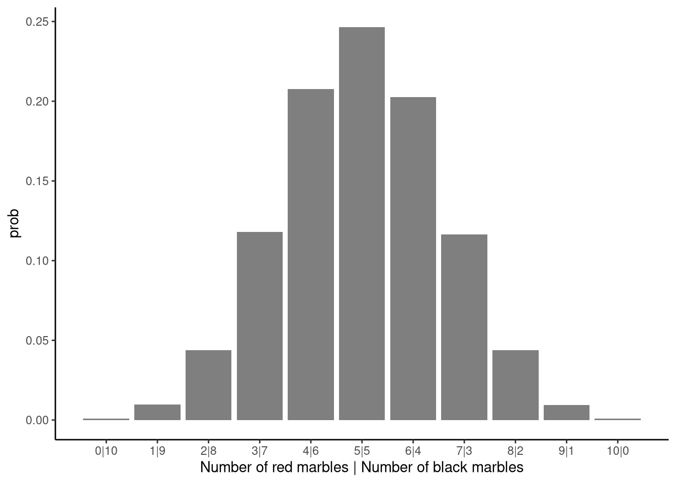
The probabilities in the prob column show how often each possible result occurred when we sampled 10 marbles from a jar with 50 red and 50 black marbles. Together, these probabilities form the sampling distribution for this particular example. In general, a sampling distribution gives the probability of each possible outcome of a sample. Notice that with 10 marbles in a sample, there are only 11 possible outcomes: 0 red and 10 black marbles, 1 red and 9 black marbles \(\ldots\) 10 red and 0 black marbles. Each of these outcomes has its own probability. Some are quite likely (for example, getting 5 red and 5 black), while others are possible but rare (such as getting all 10 marbles of the same colour).
In other words, a sampling distribution is the probability distribution of all the different results we could get from a sample. More broadly, in statistics, we use the term probability distribution to mean the set of all possible outcomes of some random process (like sampling from a jar, rolling a die, or flipping a coin) along with the probability of each outcome. A sampling distribution is just one particular kind of probability distribution, focused on the values a given sample can take.
Strictly speaking, the sampling distribution shown in Figure 4.1 is an estimate rather than the exact sampling distribution. We estimated the probabilities by repeatedly sampling taking marbles from the urn 100,000 times and calculating how often each outcome occurred. While 100,000 trials gives us a very accurate estimate, it’s still not exact due to sampling variability. In other words, if we repeated the simulation for another 100,000 samples, we would expect a slightly different estimated sampling distribution. However, for this particular problem the exact sampling distribution is known from theory. This is a binomial problem, and the exact sampling distribution follows a binomial distribution (see Note 4.3 for details).
A probability distribution assigns probabilities to each possible value of a random variable. For a six-sided die throw, the random variable \(X\) has six possible values (1–6), and the probability distribution assigns a probability to each. These probabilities must be between 0 and 1, and sum to exactly 1.
For a biased die where even faces are more likely: \[\begin{align} \begin{array}{c|rrrrrr} \hline k & 1 & 2 & 3 & 4 & 5 & 6\\ \hline \mathrm{P}\!\left(X = k\right) & 0.11 & 0.22 & 0.11 & 0.22 & 0.11 & 0.22\\ \hline \end{array} \end{align}\] where \(k\) denotes each possible value and \(\sum_{k=1}^{6} \mathrm{P}\!\left(X = k\right) = 1\). This is a probability mass function for discrete values, typically plotted as a bar chart.
Probability vs sampling distribution: The table above describes a single throw, not a statistic from repeated samples. A sampling distribution describes statistics like “number of sixes in \(n\) throws” or “mean pips across \(n\) throws.”
Continuous distributions: A random variable \(X\) can also take continuous values (time, length, speed, etc.). For continuous variables, the probability distribution is a probability density function. Because any single point has zero probability, the function gives density rather than probability. Probability densities must be non-negative, integrate to 1, but can exceed 1 at individual points. These are plotted as smooth curves.
The binomial distribution gives the probability of getting a specific number of “successes” in a fixed number of trials, where each trial has two outcomes and the success probability stays constant. For example, flipping a coin 10 times: each flip is a trial with two outcomes (heads or tails), and the binomial distribution gives the probability of getting exactly 0, 1, 2, … 10 heads.
For \(n\) trials where success has probability \(p\), the probability of exactly \(m\) successes (where \(m\) ranges from 0 to \(n\)) is: \[ \mathrm{P}\!\left(m \,\mid\,n, p\right) = \binom{n}{m} p ^ m (1-p)^{n-m}. \] The binomial coefficient \(\binom{n}{m}\) (read “\(n\) choose \(m\)”) counts the number of ways to get exactly \(m\) successes in \(n\) trials. For example, with 3 flips and 1 head, there are \(\binom{3}{1}=3\) sequences: HTT, THT, TTH.
In R, use dbinom() to calculate binomial probabilities. For example, the probability of \(m=3\) successes in \(n=10\) trials with \(p=0.6\):
dbinom(x = 3, size = 10, prob = 0.6)[1] 0.04246733The distribution’s mean is \(np\), so with \(n=10\) and \(p=0.6\), the mean is \(10 \times 0.6 = 6\) successes.
In the previous section, we discussed sampling distributions, but we have yet to describe how exactly they can be used for statistical inference. We turn to this matter now. Let us begin by showing how we can use sampling distributions to test any hypothesis about the true proportion of all young people in Britain who use illegal drugs. The result of this hypothesis test is a p-value, which is one of the most important concepts in all of inferential statistics. As we will see, a p-value is ultimately a measure of the degree of compatibility between our observed data and the hypothesis we are testing.
Although obviously highly simplified, we can formulate the drug use survey in terms of sampling from a jar of marbles. This is our statistical model for this problem (see Note 4.4). Specifically, we can treat all young people between the ages of 16 and 24 in Britain in 2017, which would have been around 5 million people, as marbles in a jar, with each marble representing a single person. The marble is red if the person it represents was taking illegal drugs (according to the definition used in the survey), or else it is black. The survey of 1,300 people can be seen as a sample of 1,300 marbles from this jar. In this sample, 172 of the marbles were red. We will also treat each marble in the sample as having been sampled with replacement. Describing the survey in this way makes it identical to the sampling from jars of marbles that we considered in Section 4.2.
All statistical inference rests on an assumed underlying mathematical model of the process that generated the data. We call this the statistical model. It is a simplified, often greatly simplified, description of a phenomenon. Models are used widely throughout science. Their purpose is to simplify complex phenomena so we can reason about or predict them. For example, the Bohr model pictures electrons orbiting a dense nucleus like planets around the sun. This is a vast simplification of atomic physics, yet it helps us conceptualise, reason, and make testable predictions. Statistical models are not only simplified descriptions; they are explicitly mathematical. They are expressed with mathematical formulae, especially probability theory.
The assumed model for the drug survey in this chapter can be likened to sampling red or black marbles from a jar with some fixed but unknown proportion of red marbles. The jar represents the population of young people in Britain; each marble is a person, red meaning the person takes illegal drugs. Drawing a sample of marbles, with replacement, represents how we obtained our survey responses. This is a drastic simplification of the true data‑generation process. Each response is made by a human who interprets the question, recalls facts, and chooses whether to be truthful. Whether someone responds at all involves further selection (joining YouGov, taking this survey). It is not clear what precise statistical population the respondents represent. Nor are the responses literally obtained by sampling with replacement. So obtaining our set of 1300 yes/no responses is not as simple as drawing marbles. Nonetheless, the model captures important features. Respondents can be viewed as a (roughly) random sample from some larger group, and each person’s yes/no response can be treated as a fixed property. Thus the urn model is a simplification that preserves key aspects, which is all any statistical model can do.
All statistical models ultimately have mathematical descriptions. In our marble-drawing analogy, the mathematical version looks like this.
Let \(n=1300\) be the total number of respondents, and let \(m=172\) be the number who report taking drugs. We’ll use \(\theta\) (pronounced theta) to represent the true proportion of drug users in the wider population — the quantity we want to learn about.
Our model assumes that \(m\) is generated by a binomial process, which describes the number of “successes” (here, people who report taking drugs) in \(n\) independent yes/no trials, each with probability \(\theta\) of success: We would write this formally as follows: \[ m \sim \textrm{Binomial}(\theta, n). \] The symbol \(\sim\) is read “is distributed as” or “is sampled from”. So we read this as “\(m\) is distributed as a binomial with parameters \(n\) and \(\theta\).” Our statistical model for the drug user proportion problem, therefore, is that \(m=172\) has been sampled from a binomial distribution of size \(n=1300\), but where we do not know the value of \(\theta\). In other words, if we could repeat the survey many times, the number of respondents saying “yes” would vary from one sample to the next according to this binomial model. The only unknown here is \(\theta\), the true proportion in the population — and statistical inference is all about using our observed \(m\) and \(n\) to learn about that unknown parameter.
Given that our drug use survey problem can be described in terms of sampling from a jar of marbles, let us consider how we would do hypothesis testing about the contents of a jar of marbles on the basis of a sample of marbles from that jar. If we sample \(n=1300\) marbles with replacement and find that \(m=172\) are red, what can we say about the true proportion of red marbles in the jar? More specifically, on the basis of this sample of \(m=172\) red marbles in a sample of \(n=1300\), how much evidence is there in favour of the hypothesis that the true proportion of red marbles in the jar is, say, 16%? There is no particular reason for choosing 16%. We are just choosing some hypothetical proportion arbitrarily as an example to start with. As we will see, the procedure that we will follow to test this hypothesis will be applicable to any and all hypotheses.
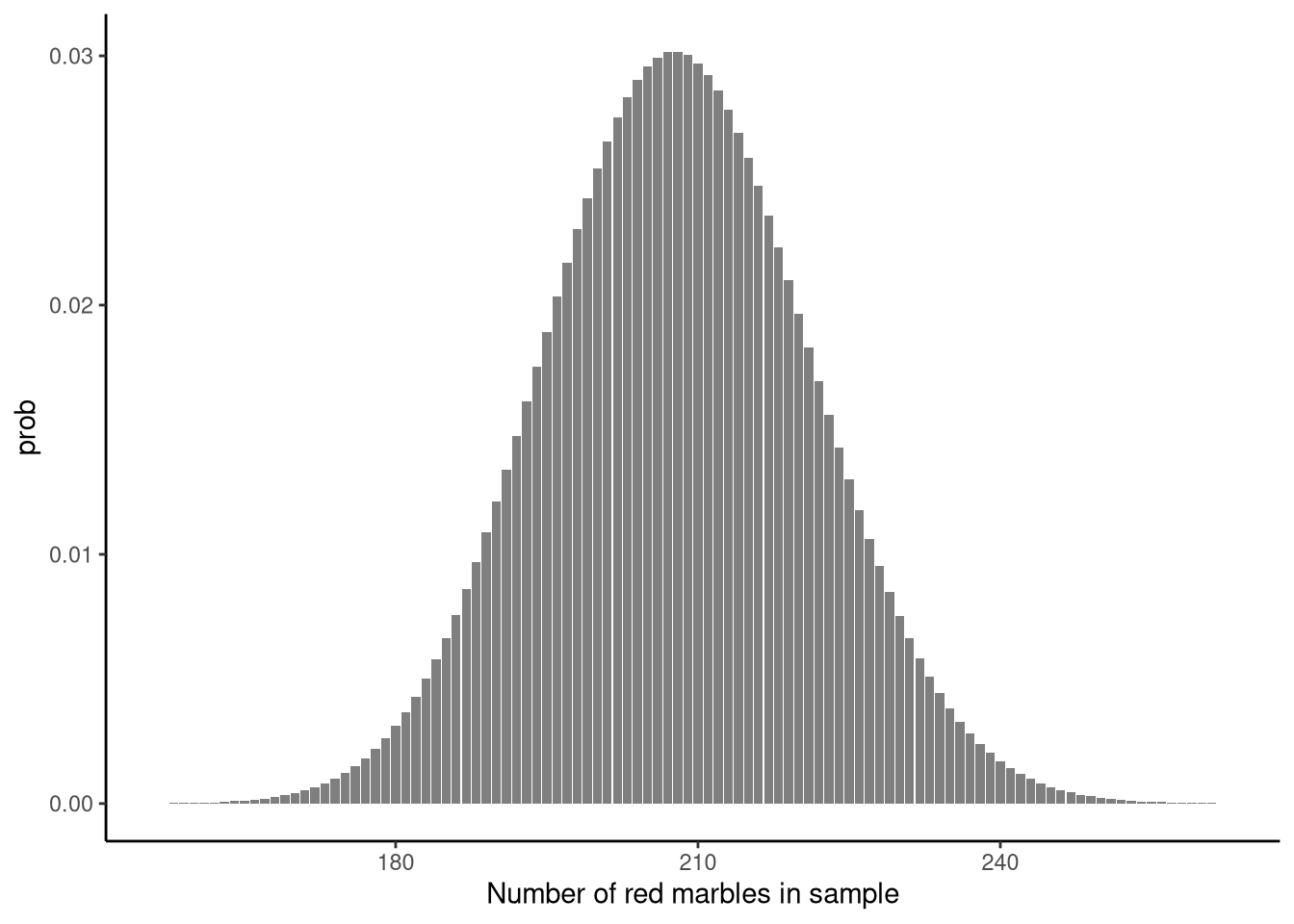
To test the hypothesis that the true proportion is 16%, we start by calculating the sampling distribution for a sample of \(n=1300\) marbles sampled with replacement from a jar whose proportion of red marbles is exactly 16%. This sampling distribution, which is shown in Figure 4.2, gives us the probability distribution over all possible values of the number of red marbles in the sample of size \(n=1300\). From that figure, we can see that the most frequent number of red marbles in the sample is around 208 and most outcomes are no more than around 25 red marbles above or below 208. In fact, we can calculate that 95% of the samples have between 182 and 234 red marbles, see Note 4.5. This simple observation is very informative: if our hypothesised proportion of 16% were true, we would rarely see samples whose number of red marbles were lower than 182 or greater than 234.
A quantile marks a point that divides a probability distribution into equal parts. A percentile is simply a quantile expressed on a 0–100 scale. For example, the 0.025 quantile is the same as the 2.5th percentile: it marks the value below which 2.5% of outcomes fall. Together, the 2.5th and 97.5th percentiles (or 0.025 and 0.975 quantiles) define the central 95% of a distribution.
For a binomial model, we can calculate these cut-offs directly in R using the function qbinom(), which returns quantiles from the binomial distribution. For example, if \(n=1300\) and \(p=0.16\), the lower and upper 95% limits for the number of red marbles can be found as follows:
qbinom(c(0.025, 0.975), size = 1300, prob = 0.16)This command asks R for the 2.5th and 97.5th percentiles of the distribution \(\mathrm{Binomial}(n=1300, p=0.16)\). The result gives the range of counts that would occur 95% of the time if the true proportion really were 15%.
In the sample that we did in fact obtain, there were 172 red marbles. This is clearly lower than 182, and so this result is not something we would have expected if the hypothesised proportion of 16% were true. Or put another way, a sample with 172 red marbles is beyond the range of probable results if the hypothesised proportion of 16% were true. If the hypothesis were true, certain results, namely a sample with between 182 and 234 red marbles, should have happened with a relatively high (around 95%) degree of probability. That did not happen, and so in that sense, this result can be said to be incompatible, or more accurately, to have a low degree of compatibility, with the hypothesis that the true proportion is 16%.
Having established that samples with between 182 and 234 red marbles occur around 95% of the time, this tells us that results lower than 182 and results higher than 234 must occur less than around 5% of the time. Results lower than 182 are in the lower tail of the distribution, and results higher than 234 are in the upper tail. These tails necessarily represent results that have a low degree of compatibility with the hypothesis. We can therefore directly quantify the degree of compatibility between any given result and the hypothesis by calculating how far into the tails any given result is. The conventional way to measure this is to first calculate how far from the centre of the sampling distribution the result is, and then calculate the tail area at or beyond any point that far from the centre. This quantity is known as a p-value. It plays an extraordinarily important role in statistics. However, its precise definition is rather subtle and elusive, and its meaning is particularly easy to misinterpret. We therefore want to introduce it very carefully here.
Let’s now calculate the p-value for the hypothesis that the true proportion is 16%, given that we observed 172 red marbles in our sample. The p-value tells us how likely it would be to obtain a result this extreme — or even more extreme — if the hypothesised proportion were actually true. For a binomial sampling distribution, the “centre” of the distribution is given by its mean, which equals the sample size multiplied by the hypothesised proportion (see Note 4.3). In our case, the sample size is \(n = 1300\) and the hypothesised proportion is 16%, so the mean of the sampling distribution is \(1300 \times 0.16 = 208\).
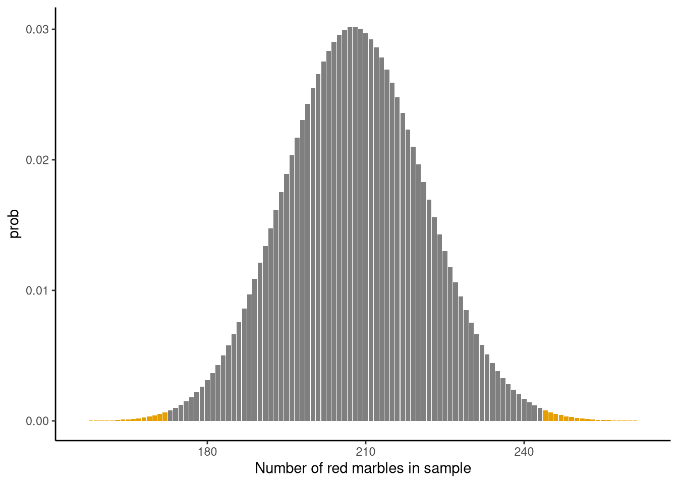
Our observed result, \(m = 172\), lies \(\|172 - 208\| = 36\) units away from that centre. (The vertical bars \(| \cdot |\) mean absolute value — we care only about how far the result is from the centre, not whether it’s above or below.) To find the p-value, we identify all outcomes that are at least this far from the centre — that is, equally or more extreme in either direction.
These two sets of outcomes are shown as the shaded tail areas in Figure 4.3.
The sum of these shaded tail areas is very low, specifically < 0.01. The sum of the probability of those tail areas — the probability of observing a result as or more extreme than ours if the hypothesised proportion were true — is the p-value, which in this case is less than (<) < 0.01. Remember that probability is measured on a 0–1 scale, where 0 means an event is impossible and 1 means it is certain. A p-value of < 0.01 therefore means that fewer than about 1% of all possible samples would be as extreme as the one we observed if the hypothesised proportion were true.
A p-value below 0.01 means that, if the hypothesised proportion of 16% were true, fewer than 1% of all possible samples would be as or more extreme than the one we observed. In practical terms, the p-value tells us how far into the tails of the sampling distribution our result lies. Specifically, low p-values correspond to results far from the centre and therefore less compatible with the hypothesis; high p-values correspond to results nearer the centre and more compatible with it. Thus, the p-value provides a measure of how compatible the observed data are with the hypothesis. What counts as “low” is a matter of convention, but the commonly used threshold is 0.05 (see Note 4.5): values at or below this are typically considered low, and values above it are not.
The p-value is the probability of obtaining a result as or more extreme than the result we observed if the hypothesis being tested is true. It tells us the degree of compatibility between the observed result and the hypothesis being tested. In general, if the p-value is low, the results have a low degree of compatibility with the hypothesis, and if the p-value is not low, the results have a higher degree of compatibility with the hypothesis. The conventional threshold delineating a “low” from a “not low” p-value is \(p = 0.05\).
We can use the binomial_pvalue() function in the sgsur package to calculate exact p-values for binomial problems. The exact p-value for the hypothesis that the true proportion of young people in Britain who take illegal drugs is exactly 16% can be obtained as follows:
binomial_pvalue(sample_size = 1300, observed = 172, hypothesis = 0.16) 0.16
0.005742506 As discussed, this p-value is low, even very low, certainly below the conventional threshold of \(p < 0.05\), and so we would conclude that there is a very low degree of compatibility between the observed results (172 drug users in a sample of 1,300) and the hypothesis that the true proportion of young people in Britain who take illegal drugs is exactly 16%. On the other hand, what about the hypothesis that the true proportion is exactly 15%? Again, we can obtain a p-value for this easily with binomial_pvalue:
binomial_pvalue(sample_size = 1300, observed = 172, hypothesis = 0.15) 0.15
0.07406892 This p-value is not particularly low — it is not below the conventional \(p=0.05\) threshold — and so we would conclude that the observed results are not incompatible with this hypothesis. Of course, that does not mean that we should now conclude that the true proportion of drug users among young people is 15%. While we will not rule out that particular hypothesis, there are many other hypotheses that we need to consider first before drawing our final conclusion. We now turn to this issue.
Thus far, we have seen how we can obtain p-values for specific hypotheses. These p-values give the degree of compatibility between the observed results and the hypothesis. If a p-value is sufficiently low, we can conclude that this effectively rules out that hypothesis. But if a p-value is not low, that does not mean that we now should consider that hypothesis as being proved correct. A p-value that is not low just means that we cannot rule it out. In general, for any problem, there will be many hypotheses that we cannot rule out. The set of all these hypotheses that we cannot rule out is known as the confidence interval.
To introduce confidence intervals, let us begin by finding the p-values for a range of hypothetical values for the true proportion of young people in Britain who take drugs. Specifically, we will look at the values from 10% to 20% in steps of 1%. We can obtain this set of values using the seq() function in R as follows:
# a sequence of values from 0.1 to 0.2 in steps of 0.01
hypotheses <- seq(0.1, 0.2, by = 0.01)
Now, we can just pass this hypotheses vector into binomial_pvalue as the value of hypothesis as follows:
binomial_pvalue(sample_size = 1300, observed = 172, hypothesis = hypotheses) |>
  round(3)
0.1 0.11 0.12 0.13 0.14 0.15 0.16 0.17 0.18 0.19 0.2
0.000 0.011 0.172 0.805 0.448 0.074 0.006 0.000 0.000 0.000 0.000 (To round the results to three decimal places, we use |> to pipe the output to the function round(3); see Section 2.6.4 for an introduction to pipes in R.) As we can see, we have obtained a range of p-values. They are low for values of 10% and 11%. At 12%, they become higher. They then drop down to low values at 16% and above. This is very informative. It tells us that the data provide a relatively high degree of support for hypothetical values of the proportion from between around 12% and 15%. Hypothetical values outside this range do not obtain much support. This gives us an approximate sense of the confidence interval.
We could go further with this approach just taken and look at a much wider range of possible values, and at a much finer grain. This would not be difficult to do, but it is not necessary. For many statistics problems, including this one, there is a mathematical formula that can identify the range of hypotheses whose p-values are all greater than some specified threshold. This is implemented in the function binomial_confint() that is part of the sgsur package. We can use it with its default settings for this problem as follows:
binomial_confint(sample_size = 1300, observed = 172) 0.025 0.975
0.1143520 0.1519436 This provides the 95% confidence interval which is the interval within which lie all hypothetical values of the proportion whose p-values are greater than 0.05. Because a p-value greater than 0.05 means that there is a relatively high, or at least not low, degree of compatibility between the data and the hypothesis, the 95% confidence interval provides the range of hypotheses that are compatible with the data. In that sense, it might be useful to call this interval a compatibility interval.
The confidence interval is the range of hypotheses not rejected by the data. A 95% confidence interval is the set of hypotheses with p‑values above 0.05. These are the hypotheses that are not incompatible with the observed data. Hypotheses outside the 95% confidence interval, on the other hand, have p‑values at or below 0.05 and so are treated as incompatible with the data. We can view confidence intervals as essentially compatibility intervals: the range of hypotheses compatible, or not incompatible, with the observed data.
In many ways then, this is the final answer to our focal question about the drug user proportion in the population of young people in Britain. From this confidence interval, we would say that the data of 172 drug users out of 1,300 provide a sufficiently high degree of support for any population proportion from 11% to 15%.
Although the 95% confidence interval is common, there is no need to always use it and we could use any level. For example, the 99% confidence interval is obtained by setting level = 0.99:
binomial_confint(sample_size = 1300, observed = 172, level = 0.99) 0.005 0.995
0.1091052 0.1582544 Every value in this range must have a p-value of at least 1%, and so we would say that any hypothetical value from 11% to 16% has at least some degree of support from the data.
A 95% confidence interval contains the true population parameter 95% of the time in repeated sampling. For example, if a jar has 60% red marbles and we repeatedly draw samples, 95% of the 95% confidence intervals we compute would contain the true value of 60%. Figure 4.4 illustrates this with 90% confidence intervals from 100 samples.
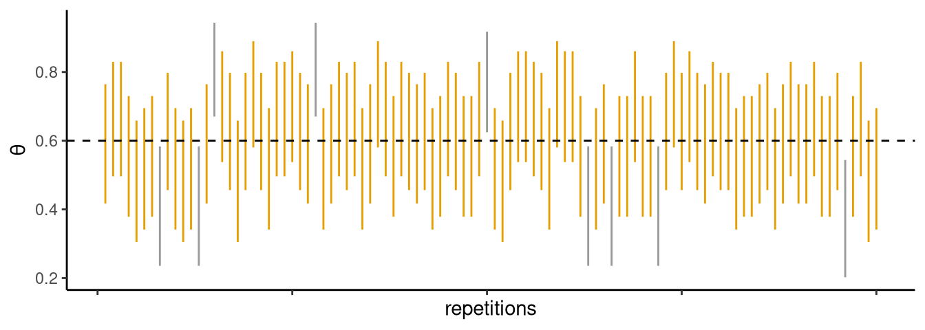
Coverage is a long-run property of the method, not a probability about any single interval. It does not mean “there is a 95% chance the true value lies in this interval” - a common misinterpretation.
More practically, interpret a confidence interval as the range of hypotheses with p-values above the chosen cutoff (e.g., p > 0.05 for a 95% interval) - the set of hypotheses reasonably compatible with the data.
In any data analysis there are usually many, or even infinitely many, hypotheses we could test. At any given moment, we often single out one particular reference hypothesis for special scrutiny; this is called the null hypothesis. It is sometimes denoted \(\mathcal{H}_0\).
What counts as the null hypothesis varies by context. Formally, it is simply the hypothesis we put “in the dock” and try to see whether the data give us reason to doubt it at the chosen p-value threshold. In practice, it is often (though not always) a “no effect” or “no important effect” hypothesis: no relationship, no difference, and so on. That familiar special case is sometimes called the nil or no‑effect hypothesis.
In our drug use example there is no uniquely obvious null hypothesis. Suppose, however, that prior global research suggested the percentage of young people worldwide who take illegal drugs is 11%. We could then take as our null hypothesis: \[
\mathcal{H}_0\colon \textsf{The proportion of young Britons who take illegal drugs is 11\%.}
\] We test \(\mathcal{H}_0\) just like any hypothesis. In this case, we would use binomial_pvalue():
binomial_pvalue(sample_size = 1300, observed = 172, hypothesis = 0.11) 0.11
0.01149416 Clearly, the p-value is relatively low, which means that the data are not compatible, or at least have a low degree of compatibility, with the null hypothesis. Using the conventional \(0.05\) threshold for p-values, we now say the data show a statistically significant difference (at the \(p < 0.05\) significance level) and that the British proportion is significantly different from the worldwide 11% figure.
The null hypothesis is the specific reference hypothesis we test for possible rejection. It is often a “no effect” hypothesis (e.g. difference = 0) but it can be any specified value or set of values chosen as the baseline. If we reject the null, we say the result is statistically significant.
Statistical significance just means that a null hypothesis has a low degree of compatibility with the data. It does not mean the result is of any scientific or practical importance, or even that it is especially noteworthy. In general, we should never mistake significance in the statistical sense with significance in the everyday sense of the term. They don’t mean the same thing. In the everyday sense of the term, a significant result would usually imply that that result has important or major practical consequences. In the statistical sense of the term, on the other hand, a significant result might correspond to a tiny or practically meaningless effect. We will encounter many situations throughout the rest of this book that highlight this distinction between statistical significance and practical significance.
Thus far, we have described exactly what a p-value is. We showed that, technically speaking, a p-value is a tail-area in the sampling distribution for a given hypothesis. In practical terms, we can treat this tail area value as a measure of the degree of compatibility between the data and a given hypothesis. The higher the p-value, the closer the result is to the centre of the sampling distribution, which means it is typical of the values we would obtain if the hypothesis were true. The lower the p-value, the further the result is into the tails of the distribution, which means it is not typical of the values we would obtain if the hypothesis were true. In this way, a p-value is a simple but useful guide as to whether a result is in line with what should happen if the hypothesis is true.
Despite the simplicity of p-values, and despite the fact that they are probably the single most fundamental concept in inferential statistics, they are widely misinterpreted and misused. They are misinterpreted and misused by students, by experienced researchers, by textbooks, and by statistics teachers. For example, see Greenland et al. (2016); Reinhart (2015); Cassidy et al. (2019); Haller & Krauss (2002); Goodman (2008) for some of the many misinterpretations and misuses of p-values and some of the contexts in which these misinterpretations arise. Some of the misinterpretations and poor practices undoubtedly arise because p-values are not described properly when they are initially introduced (as just noted, textbooks and teachers often misinterpret p-values). We have been at pains to avoid doing that in this chapter, hence our deliberately pedantic approach. But even when p-values are properly described and introduced, without constant vigilance, it seems like misunderstanding and poor practices are wont to creep back in, presumably because they are so widespread and pervasive.
The following is a list of some of the major misinterpretations and misuses of p-values.
The p-value is the probability that the null hypothesis is true. This is probably the single most egregious misinterpretation of p-values. A p-value is not the probability that the null hypothesis is true. In fact, a p-value is calculated under the assumption that the hypothesis being tested is true. A p-value is a tail area of the sampling distribution, which is the distribution over the possible results that would arise if the hypothesis being tested were true. Put another way, a p-value is the probability of obtaining results as or more extreme than the observed results, assuming the hypothesis being tested is true. As mentioned repeatedly, that probability tells us whether the observed results are compatible with what would happen if the hypothesis were true. The smaller the p-value, the less well that hypothesis would account for the observed result. It does not give the chance that the hypothesis itself is true.
The p-value is the probability that the results are due to chance alone. This is just a rephrasing of the previous misunderstanding. If the null hypothesis (of no effect in the population) is true, any pattern we see is attributable to ordinary sampling variability (“chance alone”). Saying “the results are due to chance alone” is therefore equivalent to saying “the null hypothesis is true.” But a p-value is not the probability that the null hypothesis is true. It is the probability of results as or more extreme than those observed, assuming the null hypothesis (and model) is true. Hence it is not the probability that the results are “due to chance,” but a measure of how unusual they would be if chance (as embodied in the null model) were the only explanation.
The p-value is the probability of obtaining the observed results if the hypothesis being tested is true. This is also incorrect, though much closer to the correct interpretation than any of the other misinterpretations discussed so far. The p-value gives the probability of obtaining the results, or results that are more extreme, if the hypothesis is true. For example, let us say we had a jar with red and black marbles and wanted to test if the proportion of red marbles in the jar is 50%, and let’s say we obtained 140 red marbles in a sample (sampling with replacement) of 250. If the true proportion of red marbles is 50%, the probability of exactly 140 red marbles in a sample of 250 is calculated using the binomial distribution and has a value of 0.0084 (see Note 4.3 for details about this calculation). On the other hand, given 140 red marbles in a sample of 250, the p-value for the hypothesis that the true proportion of red marbles is 50% is \(p = 0.066\). The difference between these two is that in the case of the p-value, we calculate the probability of observing 140 red marbles or any number of red marbles more extreme than that.
If the p-value for a null hypothesis is low, the null hypothesis is false. A low p-value does not logically entail that the tested hypothesis is false. It means the observed results have a low degree of compatibility with that hypothesis. Even a very small p-value is still a probability statement conditioned on the hypothesis being true, not a deductive refutation. Sampling luck, assumption violations, or hidden multiplicity can all make a true null look incompatible. A single low p-value is one piece of evidence; declaring the null “false” on that basis overstates what has been shown.
If the p-value for a null hypothesis is low, we should conclude that there is an effect (e.g., association, difference between groups) in the population. A low p-value is evidence against the specific no‑effect (or reference) hypothesis, but by itself it does not establish that a real population effect exists, nor its size, importance, direction, stability, or cause. Such a result could arise from modelling misspecification or bias of various kinds, or just simple chance among many research attempts. Even under ideal conditions, one statistically significant study gives limited confirmation: it shows incompatibility with one hypothesis, not a well‑characterised alternative. Fisher himself warned that “no isolated experiment, however significant in itself, can suffice for the experimental demonstration of any natural phenomenon,” and that a phenomenon is “experimentally demonstrable” only when an experiment will reliably yield significance (Fisher, 1935, p. p16). Thus a low p-value is a starting signal for replication and estimation, not a final verdict that a meaningful effect has been established.
A low p‑value provides strong evidence in favour of the hypothesis being tested. A p‑value gauges how well the data line up with the tested hypothesis; the smaller it is, the less well the hypothesis accounts for the data. Thus a low p‑value is evidence against that hypothesis, not for it. Confusion arises because the hypothesis under test is often a “no‑effect” statement, so researchers wishing to show an effect mentally swap in the alternative when they read “hypothesis.” Always keep track of which hypothesis the p‑value is calculated under: a small p-value means low compatibility with that hypothesis, a large p-value means high compatibility.
A p-value is interpreted only by checking whether it is above or below a threshold such as \(p=0.05\). A p-value is a continuous measure of how compatible the data are with the tested hypothesis. Higher values indicate greater compatibility; lower values indicate less. Interpret the number on its own scale, not just by the side of an arbitrary cut‑off it falls on. Except when it is extremely small (say <0.001), report the exact value, e.g., \(p=0.085\), \(p=0.54\), \(p=0.023\), not merely \(p<0.05\) or \(p>0.05\). Treating, for example, \(p=0.25\) and \(p=0.57\) as equivalent, throws away meaningful information. Likewise, a result with \(p=0.04\) should not prompt a categorically different conclusion from one with \(p=0.06\); the change in compatibility is tiny. The American Statistical Association’s 2016 statement makes this point explicitly: “Scientific conclusions and business or policy decisions should not be based only on whether a p‑value passes a specific threshold” (Wasserstein & Lazar, 2016). Sound inference also weighs study design, measurement quality, external evidence, and the validity of model assumptions, not the p‑value alone.
Greenland et al.’s “Statistical tests, P values, confidence intervals, and power: a guide to misinterpretations” (Greenland et al., 2016) provides a clear, authoritative summary of what p-values and confidence intervals do not mean.
Alex Reinhart’s Statistics Done Wrong (Reinhart, 2015) offers a humorous but serious examination of common inferential mistakes, particularly valuable for students new to hypothesis testing.
Gelman and Stern’s “The difference between ‘significant’ and ‘not significant’ is not itself statistically significant” (Gelman & Stern, 2006) illustrates the dangers of dichotomous thinking about p-values in a concise paper from The American Statistician.