13 Models for count data
Many psychological and social phenomena involve outcomes that count how often something occurs — the number of panic attacks in a month, aggressive acts during an observation period, or times a student seeks academic support. These are counts rather than continuous measures, and they often show distinctive statistical patterns: many zeros, no negative values, and a tendency for the variability to grow with the mean. Ordinary linear regression cannot handle such data appropriately because it assumes normally distributed residuals and allows for impossible predictions such as negative counts. To analyse these outcomes, we need models that explicitly account for their discrete and non-negative nature. This chapter introduces such models. Building on the framework of generalised linear models from Chapter 12, we’ll explore how the Poisson and related distributions can be used to model count outcomes, handle overdispersion, and account for data with excess zeros or unequal exposure.
The chapter covers
- Count data represent non-negative integers recording event frequencies, requiring models that respect their discrete nature and prevent impossible negative predictions.
- Poisson regression models counts using a log link, with the key assumption that mean and variance are equal.
- Overdispersion occurs when variance exceeds the mean, violating Poisson assumptions and requiring quasi-Poisson or negative binomial alternatives.
- Negative binomial regression relaxes the Poisson’s mean-variance constraint by introducing an additional dispersion parameter.
- Zero-inflated models handle excess zeros by combining a process generating structural zeros with a count process for non-zero values.
- Offset terms adjust for variable exposure periods, allowing models to estimate rates rather than raw counts when observation windows differ.
13.1 Poisson Regression
Having outlined the purpose and scope of this chapter, we now turn to the foundations of count modelling — beginning with the Poisson distribution, which provides the simplest model for counts within a fixed time or space interval. The Poisson distribution models the number of times something has happened. It has just one parameter: \(\lambda\) (lambda), which is also known as the rate parameter, or simply the rate. The value of \(\lambda\) describes both the mean of the Poisson distribution and its variance. An important consequence of this is as one increases so does the other. In other words, we would expect a sample drawn from a Poisson distribution that has a large mean would also have a large variance. Note also that while count data may only take on non-negative integer values, \(\lambda\) itself does not have this constraint, and hence may take on any non-negative value. This is because \(\lambda\) represents the mean (or variance) of the distribution, and the mean number of times something happened can and will usually be a non-integer, though it must still be non-negative.
Let’s look at an example. We are interested in how many times 5 people visit the doctor in a year and record the following data, with one data point from each individual: \[ 2, 0, 1, 1, 5 \] Each individual data point is a non-negative integer value, but if we were interested in the mean number of times individuals in this sample visited the doctor, our result is the non-integer value \((2+0+1+1+5)/5 = 1.8\). Since \(\lambda\) represents the mean of the Poisson distribution and in turn the mean of the counts in the population, it makes sense that it does not necessarily have to take on a discrete value; it will, however, always be non-negative.
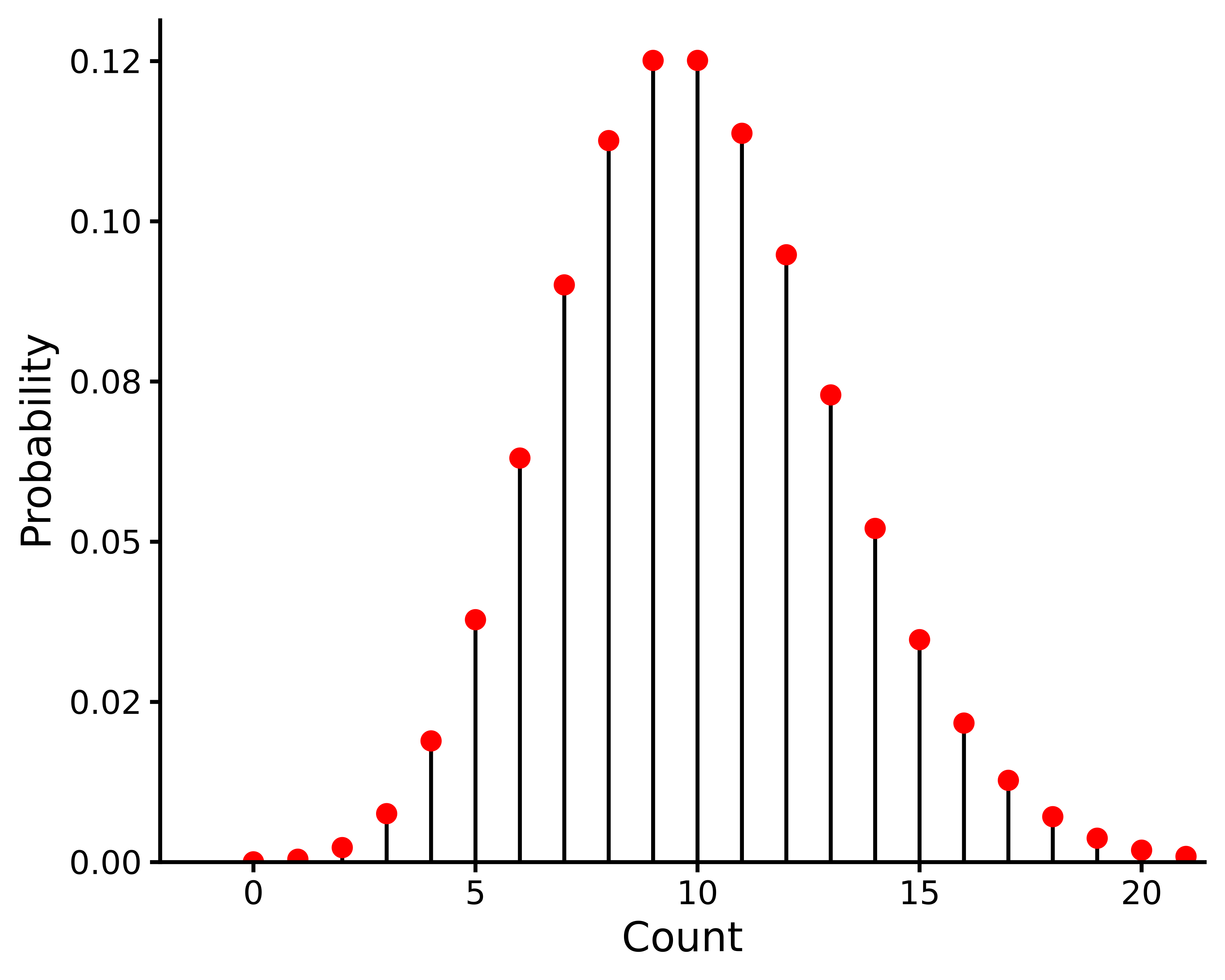
The Poisson distribution takes different shapes for different values of \(\lambda\), as illustrated in Figure 13.1. This visualises the relationship between the mean and the variance in this distribution; when \(\lambda\) is low, both the mean and the variance of the data are low, and when \(\lambda\) is large, the mean and the variance are both large.
In summary, if our outcome variable is a count variable, an appropriate distribution with which to model it is the Poisson. The \(\lambda\) of this distribution is unknown and is something that we can establish from our model. If we choose the Poisson distribution for our outcome variable and want to model it as a function of a predictor or a set of predictors, then we need to use Poisson Regression.
In the previous chapter, we discussed that generalised linear models have three key components:
- The probabilistic family. This specifies the distribution for the outcome variable, the location parameter of which varies as a function of explanatory variables.
- The deterministic component, or linear model. This defines how the main parameter, or its transformation, varies as a function of the predictor variables.
- A link function. This specifies the transformation that is applied to the location parameter of the outcome variable’s probability distribution.
In Poisson regression, we assume that the outcome variable follows a Poisson distribution whose location parameter is \(\lambda\) and the default link function applied to the Poisson distribution is the \(\log\) link. We have already seen the \(\log\) function; see Note 3.2. There, we saw that the inverse of the \(\log\) is the exponential function \(e^{(\cdot)}\), which is sometimes written \(\exp(\cdot)\).
The Poisson regression model is therefore as follows: \[ \begin{aligned} y_i &\sim \textrm{Poisson}(\lambda_i),\quad\text{for $i \in 1, 2 \ldots n$},\\ \log(\lambda_i) &= \beta_0 + \sum_{k=1}^K \beta_k x_{ki}. \end{aligned} \] As we can see, the logarithm of \(\lambda_i\), and not \(\lambda_i\) itself, is a linear function of the \(\vec{x}_i\). The reason for this is that \(\lambda_i\) must be non-negative. Were \(\lambda_i\) to vary as a linear function of \(\vec{x}_i\), it is possible that it could have negative values, which would be meaningless. However, \(\log(\lambda_i)\) takes values on the real line from \(-\infty\) to \(\infty\), and so regardless of the coefficients of the linear model, and regardless of the values of the \(\vec{x}_i\), the value of \(\log(\lambda_i)\) will always be meaningful. Because our link functions must be invertible, for any value of \(\log(\lambda_i)\) we can obtain \(\lambda_i\) by applying the inverse link function to \(\log(\lambda_i)\) as follows: \[ \lambda_i = \exp(\log(\lambda_i)). \]
13.2 Poisson regression in R
To explore Poisson regression, we’ll use the nhanes1112 dataset from sgsur, which details health information for 3361 individuals. Our outcome variable will be DaysPhysHlthBad, which represents the number of days a participant reported their health not being good in the previous 30 days. Note here that the variable is a count, i.e., it is the number of times something happened, i.e., someone reported not having good health, and it is in a fixed time interval, 30 days. These two elements are essential for the data to be analysed using a Poisson regression (although see Section 13.4 for how we can manage count data that is not recorded in a fixed time interval). Our predictor variable will be age of the participant, recorded in years. This data is shown in Figure 13.2.
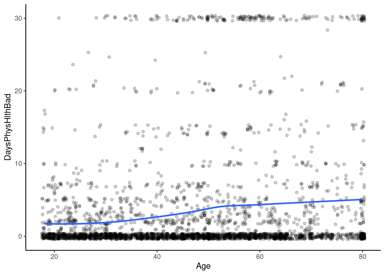
Here, we see that whilst the number of bad physical health days increases with age, it does so in a non-linear way; we see that around age 40 the slope of the line becomes slightly steeper and then begins to plateau out around age 60 or so. Visualising this relationship here is instructive since it helps us to see that we do not, in this case at least, have a linear relationship between age and the number of self-reported days of bad physical health.
Let’s run the model in R.
M_13_1 <- glm(DaysPhysHlthBad ~ Age,
                        data = nhanes1112,
                        family = poisson(link = "log"))
Using our glm() function, we specify the outcome, the predictor and the data. Finally, we specify the family, or type of generalised linear model we want to run; here that is the Poisson model, and we specify that the link is log, i.e., that we want to transform the outcome variable using a logarithm before we use it in the model.
We can access the model output as usual:
summary(M_13_1)
Call:
glm(formula = DaysPhysHlthBad ~ Age, family = poisson(link = "log"),
    data = nhanes1112)

Coefficients:
             Estimate Std. Error z value Pr(>|z|)
(Intercept) 0.1798052  0.0305152   5.892 3.81e-09 ***
Age         0.0199822  0.0005454  36.639  < 2e-16 ***
---
Signif. codes:  0 '***' 0.001 '**' 0.01 '*' 0.05 '.' 0.1 ' ' 1

(Dispersion parameter for poisson family taken to be 1)

    Null deviance: 33722  on 3352  degrees of freedom
Residual deviance: 32362  on 3351  degrees of freedom
  (8 observations deleted due to missingness)
AIC: 36467

Number of Fisher Scoring iterations: 6
First, we’ll extract the model coefficients along with their 95% confidence intervals:
coef(M_13_1)(Intercept) Age
0.17980515 0.01998216 confint(M_13_1) 2.5 % 97.5 %
(Intercept) 0.11979548 0.23942072
Age 0.01891385 0.02105181We interpret these the same way as any linear model: the intercept represents the predicted log of the average number of bad health days when the predictor, age, is zero. The slope shows the predicted increase in the log of the average when bad health days increase by one. What is important to remember here, though, is that these values are logarithms of averages. As such we can exponentiate them to return to the original count scale.
exp(coef(M_13_1))(Intercept) Age
1.196984 1.020183 The intercept (exp(0.18) ≈ 1.20) represents an expected average of about 1.2 bad health days when age is zero. The slope (exp(0.02) ≈ 1.02) indicates that for each additional year of age, the expected number of bad health days increases by a factor of 1.02 — roughly a 2% rise per year.
Let’s make some predictions using these coefficients first, and then we’ll look at how to transform them back to counts.
First, we specify the age range we want to use as predictions, and can then calculate our predictions of the log of an individual reporting bad health days based on their age:
newdata <- data.frame(Age = seq(18, 75, by = 1))

#| echo: true
nhanes_predictions <- newdata |>
  mutate(predicted_bad_health = predict(M_13_1, newdata = newdata))

head(nhanes_predictions)
Age predicted_bad_health
1 18 0.5394840
2 19 0.5594662
3 20 0.5794483
4 21 0.5994305
5 22 0.6194126
6 23 0.6393948Looking at these predictions, we can see that based on our model, we would predict the logarithm of the counts to be 0.6 for a 21-year-old.
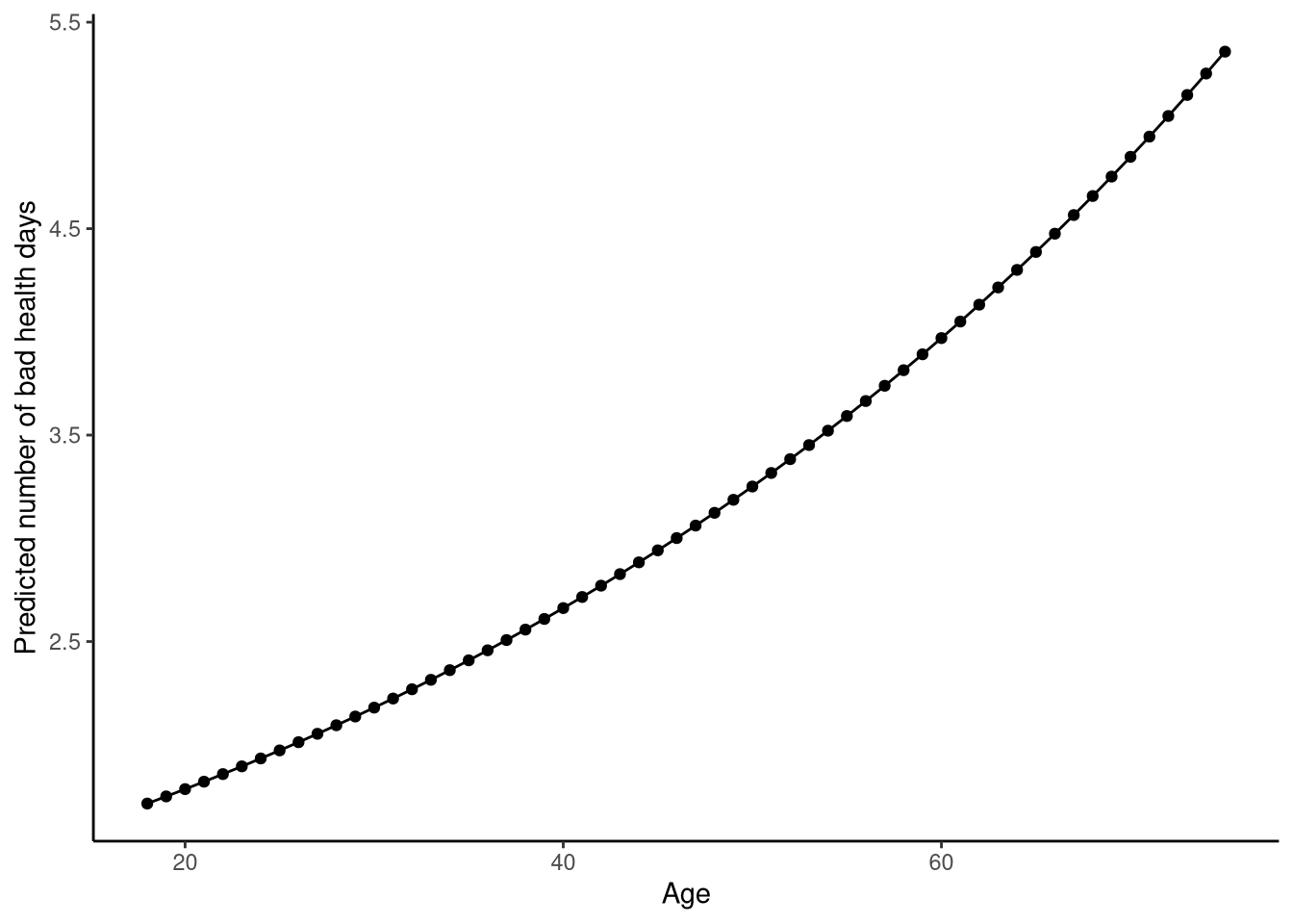
To make these predictions easier to interpret, we can transform them back to counts using exponentiation This mathematical function allows us to undo the logarithm and turn the predictions back to the original units, counts:
nhanes_predictions <- newdata |>
  mutate(predicted_bad_health = predict(M_13_1, newdata = newdata)) |>
  mutate(predicted_bad_health = exp(predicted_bad_health))

head(nhanes_predictions)
Age predicted_bad_health
1 18 1.715122
2 19 1.749738
3 20 1.785053
4 21 1.821081
5 22 1.857836
6 23 1.895333These predictions are shown in Figure 13.3.
Now that we have an idea of the relationship between age and bad health days, let’s take a look at the hypothesis tests associated with our model:
summary(M_13_1)$coefficients Estimate Std. Error z value Pr(>|z|)
(Intercept) 0.17980515 0.0305151522 5.892324 3.808025e-09
Age 0.01998216 0.0005453756 36.639258 6.785150e-294We can see that the p-value associated with the slope coefficient is less than 0.05, and hence we can conclude that it is very unlikely that we would have obtained this result, or a result more extreme, if in fact the relationship between age and bad health days is zero.
13.2.1 Overdispersion
Above, we noted that one of the properties of the Poisson model is that its mean and its variance are identical. Data generated by a Poisson distribution should have sample means and sample variances that are very close to one another. This is known as equidispersion.
Remember that we assume that count data is drawn from a Poisson distribution in the population — we describe this in our formal definition of the model as \[y_i \sim \text{Poisson}(\lambda_i),\] that each observation is drawn from a Poisson distribution and that this distribution is measured by one parameter, \(\lambda_i\). In the Poisson distribution, \(\lambda\) represents both the mean and the variance, and hence the variance cannot be modelled separately from the mean, as is the case in, say, a normal distribution, where we have a parameter for the mean (\(\mu\)) and a parameter for the variance (\(\sigma^2\)). This means that the value of the mean and the variance in a Poisson distribution are linked; for example, as the mean increases, so does the variance, i.e., if the mean of the distribution is 3 then we would expect the variance of the distribution to also be 3. This logic applies to any samples that we assume are drawn from a Poisson distribution; we expect that their mean and variance are approximately equal. Because of this assumption, we must check that the mean and variance in our sample of count data are approximately equal. If we find that the variance is larger than the mean, or that the variance is smaller than the mean, our data would be overdispersed or underdispersed. In other words, it would not meet the assumption of equidispersion. Overdispersion causes the standard errors to be underestimated in the model, whilst underdispersion overestimates them. Underestimating the standard errors is problematic, since it can cause an overestimation of the test statistic leading to erroneous conclusions about the significance and confidence and credible intervals.
Let’s first examine the dispersion in our sample, and then we will discuss ways to handle over- or underdispersed data. First, let’s calculate the mean and variance of our count variable, the number of poor health days in the previous 30 days:
nhanes1112 |>
  summarise(mean = mean(DaysPhysHlthBad, na.rm = T),
            variance = var(DaysPhysHlthBad, na.rm = T))
# A tibble: 1 × 2
mean variance
<dbl> <dbl>
1 3.25 53.8Clearly, the variance is far higher than the mean, and we can conclude that our data are overdispersed and hence the model does not meet the assumption of equidispersion.
Note 13.1: Dealing with Overdispersion: Quasi-Poisson
A quick, though not especially principled, way to handle overdispersion is to use a quasi-Poisson model. This model assumes that the variance is proportional to the mean:
\[ \text{Var}(Y_i) = \phi \, \mu_i \]
where \(\phi\) is the overdispersion parameter (estimated from the data) and equals 1 under the standard Poisson model. Standard errors are then adjusted by this parameter:
\[ \text{SE}_{\text{quasi}} = \sqrt{\phi} \, \text{SE}_{\text{Poisson}} \]
In R, we can fit this model simply by specifying family = quasipoisson:
Although this corrects the standard errors, it does not model the source of overdispersion — it only compensates for it. A more principled alternative is to use a distribution, such as the negative binomial, that explicitly allows the variance to vary separately from the mean.
13.3 Negative binomial regression
Remember that our Poisson distribution assumes that the mean and variance are equal (equidispersion). A more flexible way to handle overdispersion is to use a probability distribution that allows the variance to be modelled separately from the mean — the negative binomial distribution.
This distribution is defined by two parameters: the mean \(\mu\) and a shape (or dispersion) parameter \(\theta\). Like the Poisson, it models discrete, non-negative counts.
Formally, the negative binomial model assumes:
\[ Y_i \sim \text{NegBin}(\mu_i, \theta), \qquad \text{Var}(Y_i) = \mu_i + \frac{\mu_i^2}{\theta} \] This means that the expected value of \(Y_i\) is still \(\mu_i\), as in the Poisson model, but the variance now depends on both the mean and the parameter \(\theta\). When \(\theta\) is small, the second term \(\mu_i^2 / \theta\) becomes large, introducing extra variability (overdispersion). As \(\theta\) increases, the extra variance term shrinks, and when \(\theta \to \infty\) the variance equals the mean and the model reduces to a standard Poisson model.
As such, the Poisson distribution can in fact be thought of as a special case of the negative binomial. This is beneficial since if we do not have overdispersion in our data but use the negative binomial distribution in our model, our results will approximate those from a model with a Poisson distribution.
The linear predictor follows the same log link as the Poisson:
\[ \log(\mu_i) = \beta_0 + \beta_1 X_i \]
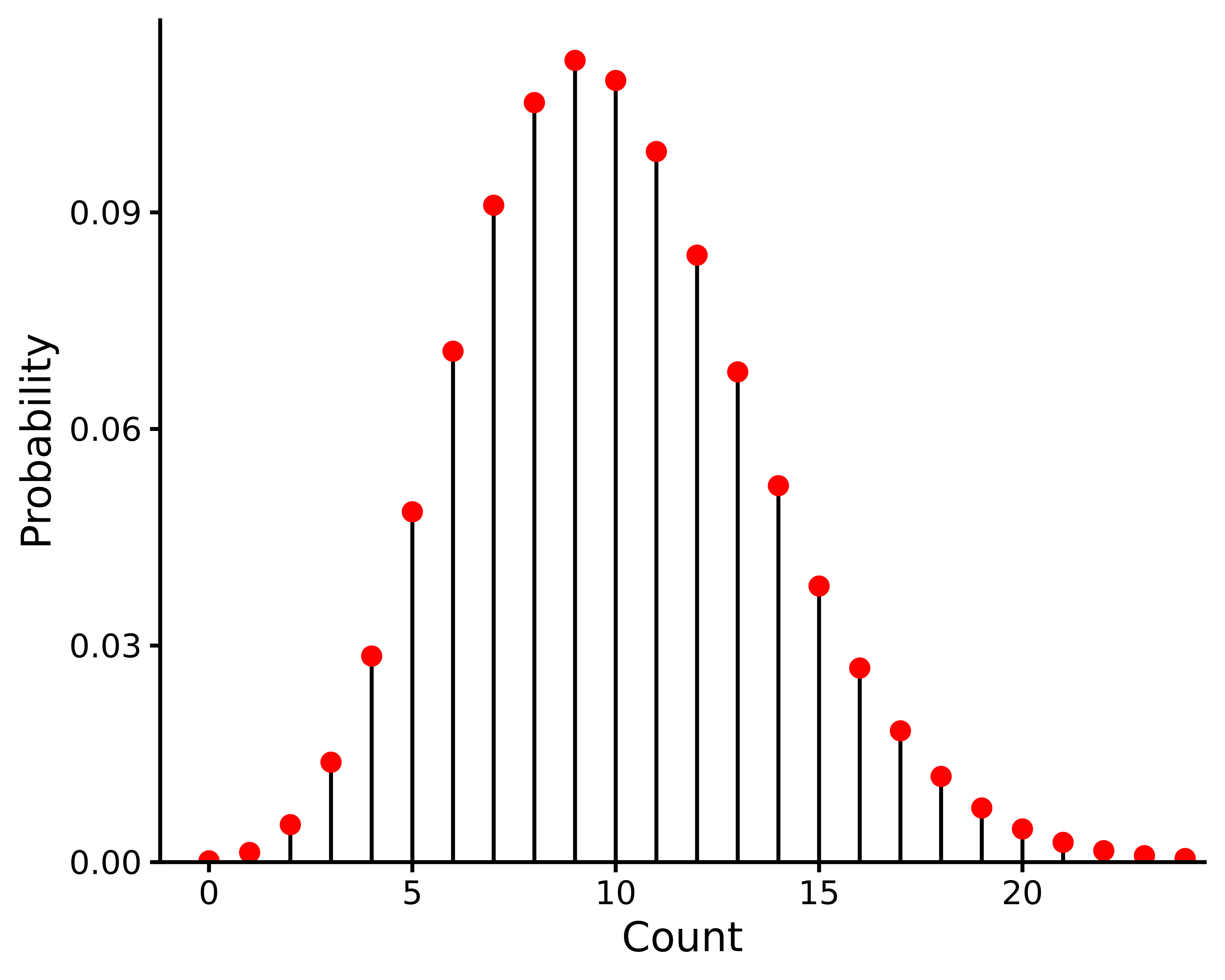
The negative binomial distribution is illustrated in Figure 13.4 for representative parameter values.
Let’s move to fitting and interpreting the negative binomial regression in R. We’ll use the glm.nb function from the sgsur package (re-exported from MASS), and we’ll keep working to predict bad health days by age.
M_13_2 <- glm.nb(DaysPhysHlthBad ~ Age, data = nhanes1112)And we’ll examine the results
summary(M_13_2)
Call:
glm.nb(formula = DaysPhysHlthBad ~ Age, data = nhanes1112, init.theta = 0.1368623043,
    link = log)

Coefficients:
            Estimate Std. Error z value Pr(>|z|)
(Intercept) 0.092326   0.136557   0.676    0.499
Age         0.021728   0.002712   8.012 1.13e-15 ***
---
Signif. codes:  0 '***' 0.001 '**' 0.01 '*' 0.05 '.' 0.1 ' ' 1

(Dispersion parameter for Negative Binomial(0.1369) family taken to be 1)

    Null deviance: 2373.1  on 3352  degrees of freedom
Residual deviance: 2313.2  on 3351  degrees of freedom
  (8 observations deleted due to missingness)
AIC: 11584

Number of Fisher Scoring iterations: 1

              Theta:  0.13686
          Std. Err.:  0.00511

 2 x log-likelihood:  -11578.32400
Similar to the Poisson regression, the coefficients are interpreted in terms of the logarithms of the average outcome. Focusing on the model coefficients along with their 95% confidence intervals, we see that the log count of the average number of bad health days when age is zero is approximately 0.18 and that for every one unit increase in age, the log of the average number of bad health days increases by 0.02. Exponentiating these coefficients transforms them back to the count scale: exp(0.18) ≈ 1.20 represents an expected average of 1.2 bad health days when age is zero, and exp(0.02) ≈ 1.02 indicates that for each additional year of age, the expected number of bad health days increases by about 2%.
coef(M_13_1)[1](Intercept)
0.1798052 confint(M_13_1) 2.5 % 97.5 %
(Intercept) 0.11979548 0.23942072
Age 0.01891385 0.02105181Just as with the Poisson model, we can use the model coefficients to make predictions, and exponentiate these to return them to the count scale:
newdata <- tibble(Age = seq(18, 75, by = 1))

#| echo: true
nhanes_predictions_nb <- newdata |>
  mutate(predicted_bad_health = predict(M_13_2,
    newdata = newdata
  )) |>
  mutate(predicted_bad_health = exp(predicted_bad_health))

head(nhanes_predictions_nb)
# A tibble: 6 × 2
Age predicted_bad_health
<dbl> <dbl>
1 18 1.62
2 19 1.66
3 20 1.69
4 21 1.73
5 22 1.77
6 23 1.8113.4 Zero-inflation
When we work with count data, there is the possibility that the number of times something happened is zero. Sometimes find far more zeros than expected under a standard Poisson or negative binomial distribution — a pattern known as zero inflation.
We can assess this qualitatively by examining our data. Let’s use the nhanes1112 dataset and focus on the variable AlcoholYear. The variable details the estimated number of days in the last year that an individual drank an alcoholic beverage.
We can see how many of these are zeros using count():
count(nhanes1112, AlcoholYear)# A tibble: 45 × 2
AlcoholYear n
<int> <int>
1 0 487
2 1 111
3 2 101
4 3 105
5 4 56
6 5 84
7 6 65
8 7 6
9 8 9
10 9 1
# ℹ 35 more rowsThis shows us that 487 observations were zero. That is, 487 individuals in the dataset reported zero days of drinking alcohol in the last year.
Conceptually, it can be helpful to think of these zeros as arising from two different processes. Some individuals produce structural zeros — for example, people who never drink alcohol and therefore have a probability of one of recording zero drinking days. Others produce sampling zeros (also called stochastic or occasional zeros) — people who do drink, but happened not to do so in the past year.
Although we cannot directly identify which individuals belong to which group, we can represent this idea statistically by assuming that a latent process determines whether an observation comes from the always-zero group or from the regular count-generating process. Importantly, the count process itself can also produce zeros, meaning that in a zero-inflated model some zeros come from the always-zero group while others arise naturally from the count distribution. This mixture of two sources of zeros is what distinguishes zero-inflated models from hurdle models (see Note 13.2), where all zeros are assumed to come from a single process.
Note 13.2: Hurdle Models
A hurdle model provides another way to handle excess zeros, but it makes a different assumption from the zero-inflated model.
In a zero-inflated model, zeros can arise from two sources: 1. A separate process that always produces zeros (e.g. people who never drink alcohol). 2. The regular count process (e.g. occasional drinkers who happened not to drink this year).
In contrast, a hurdle model assumes that all zeros come from a single binary process that determines whether the “hurdle” is crossed. Once the hurdle is crossed (i.e. the count is positive), a second model describes the size of the count, using a truncated count distribution (where zeros are excluded).
Mathematically, this means: - A binary model (often logistic) predicts whether \(Y_i = 0\) or \(Y_i > 0\). - A count model (Poisson, negative binomial, etc.) is fitted only to \(Y_i > 0\).
Hurdle models are especially useful when zeros represent a qualitatively different process — for example, the decision to start doing something (drinking, exercising, offending) is separate from how often it is done.
13.4.1 Zero-inflated Poisson
The zero-inflated Poisson (ZIP) model combines two components: 1. A zero-model describing the probability that an observation comes from the structural zero process. 2. A Poisson count model describing the expected counts for the remaining observations, which may include both sampling zeros and positive counts.
Together, these form a mixture model — a probabilistic model that combines multiple underlying processes. Here, we define a latent variable \(z_i \in \{0, 1\}\) to indicate whether an observation belongs to the structural-zero process \(( z_i = 0 )\) or to the count process ($ z_i = 1 $).
The formal definition of the zero-inflated Poisson is as follows, where we have a count outcome variable \(y_i\), a predictor \(x_i\), and a latent variable \(z_i\) which can take on the values {0,1}, that determines whether each observation arises from the structural-zero process or the count-generating process.
Formally, this mixture model is as follows: \[ \begin{aligned} y_i &\sim \begin{cases} \textrm{Poisson}(\lambda_i), &\quad\text{if $z_i = 0$},\\ \mathbb{I}(0), &\quad\text{if $z_i = 1$} \end{cases},\\ z_i &\sim \textrm{Bernoulli}(\theta_i) \end{aligned} \]
Here, the \(z_i \in \{0, 1\}\) is the latent variable that indicates whether the observation belongs to the structural-zero process (\(z_i = 1\)) or the count-generating process (\(z_i = 0\)). The notation \(\mathbb{I}(0)\) denotes a degenerate distribution that takes the value zero with probability one — in this model, it represents the structural-zero component, the part of the mixture that always produces zeros regardless of the predictors.
The value of \(\theta_i\) gives the probability that \(z_i = 1\). This probability varies as a function of the predictors just like in a binary logistic regression: \[ \log\left(\frac{\theta_i}{1 - \theta_i}\right) = \beta_0 + \sum_{k=1}^{K} \beta_k x_{ki}. \] Likewise, the mean of the count component, \(\lambda_i\), varies as a function of the predictors, just like in a Poisson regression. \[ \log(\lambda_i) = \gamma_0 + \sum_{k=1}^K \gamma_k x_{ki}. \] In other words, the outcome variable $ y_i $ is drawn from a Poisson distribution when the latent variable indicates membership in the count process (\(z_i = 0\)), and takes the value zero when the latent variable indicates membership in the structural-zero process ($z_i = 1 $). The latent Bernoulli variable \(z_i\) therefore determines which of the two processes — structural zero or count-generating — produces each observation.
Note 13.3: Zero-Inflated Negative Binomial
A zero-inflated negative binomial (ZINB) model extends the logic of the zero-inflated Poisson to situations where the count data are also overdispersed — that is, when the variance exceeds the mean.
The model has the same two components as the ZIP: 1. A zero-model describing the probability of belonging to the structural-zero process. 2. A count model, but now using a negative binomial distribution instead of a Poisson.
This allows the model to handle both excess zeros and overdispersion at the same time, making it a more flexible alternative when the Poisson assumption of equidispersion does not hold.
13.4.2 Zero-inflated Poisson Regression in R
In this example, we’ll use the zeroinfl function from the sgsur package (re-exported from the pscl package), and we’ll continue with our example above and explore the count of alcoholic drinks consumed in a year as a function of age. We specify the model as follows:
M_13_3 <- zeroinfl(AlcoholYear ~ Age, data = nhanes1112)We can assess the model output using summary()
summary(M_13_3)
Call:
zeroinfl(formula = AlcoholYear ~ Age, data = nhanes1112)

Pearson residuals:
   Min     1Q Median     3Q    Max
-3.327 -1.997 -1.389  1.246 14.804

Count model coefficients (poisson with log link):
             Estimate Std. Error z value Pr(>|z|)
(Intercept) 3.8150035  0.0063888   597.1   <2e-16 ***
Age         0.0144125  0.0001224   117.7   <2e-16 ***

Zero-inflation model coefficients (binomial with logit link):
             Estimate Std. Error z value Pr(>|z|)
(Intercept) -3.196567   0.165216  -19.35   <2e-16 ***
Age          0.031489   0.002991   10.53   <2e-16 ***
---
Signif. codes:  0 '***' 0.001 '**' 0.01 '*' 0.05 '.' 0.1 ' ' 1

Number of iterations in BFGS optimization: 9
Log-likelihood: -1.405e+05 on 4 Df
Before the coefficient blocks, we see the Pearson residuals. These values summarise the difference between the observed and expected counts, scaled by the model’s expected variance. Large positive or negative residuals indicate observations where the model substantially over- or under-predicts the count. In our output, the residuals range from approximately -3.3 to 14.8, suggesting that a few cases are poorly fitted by the model — a common sign of overdispersion or unmodelled structure in count data.
Looking further down, we find two blocks of coefficients: the first corresponds to the count model (the Poisson component), and the second to the zero-inflation model (the binary logistic component). The count component provides estimates for predictors of the expected counts, while the logistic component models the probability of belonging to the structural-zero process rather than the count-generating process.
Let’s first focus on the count model coefficients:
summary(M_13_3)$coef$count Estimate Std. Error z value Pr(>|z|)
(Intercept) 3.81500348 0.0063887997 597.1393 0
Age 0.01441249 0.0001224079 117.7415 0We interpret these coefficients as we would for any Poisson model, remembering that they apply only to the count-generating process (the individuals not in the structural-zero group).
We have an intercept and a slope, both expressed in terms of log averages of counts. The positive slope indicates that as age increases, so does the number of days alcoholic drinks were consumed within a year. Specifically, each one-year increase in age corresponds to an increase in the log of the expected count by 0.014.
Exponentiating the coefficients returns them to the original count scale. The intercept, exp(3.82) ≈ 45.5, represents the expected number of drinking days per year for an individual aged zero — not meaningful in itself but useful as a baseline for scaling. The slope, exp(0.014) ≈ 1.015, means that for each additional year of age, the expected number of drinking days increases by a factor of about 1.5%, among those in the count-generating group.
We can also see that the slope coefficient is statistically significant, such that it is very unlikely that we would have obtained these results, or results more extreme, if the relationship between the number of days alcoholic drinks were consumed in a year and age was zero in the population.
Now let’s move to the zero-inflation component of the model:
summary(M_13_3)$coef$zero Estimate Std. Error z value Pr(>|z|)
(Intercept) -3.19656661 0.165216408 -19.34776 2.129157e-83
Age 0.03148922 0.002990689 10.52909 6.344607e-26This part of the model predicts the probability that an individual belongs to the structural-zero process — that is, the group who always report zero drinking days — as opposed to the count-generating process. The coefficients are expressed in log odds, as in any binary logistic regression. The positive slope indicates that as age increases, so does the log odds of belonging to the structural-zero group. Specifically, for every one-year increase in age, the log odds increase by 0.031. The exponentiated slope, exp(0.031) ≈ 1.03, means that each additional year of age increases the odds of being in the structural-zero group by about 3%, holding other predictors constant. We can also transform the intercept to the probability scale using the logistic function, plogis(-3.2) ≈ 0.039, which means that when all predictors are set to zero, the model estimates roughly a 4% probability of belonging to the structural-zero group.
Note that we can obtain 95% confidence intervals for all coefficients in the model using confint():
confint(M_13_3) 2.5 % 97.5 %
count_(Intercept) 3.80248166 3.82752530
count_Age 0.01417258 0.01465241
zero_(Intercept) -3.52038482 -2.87274840
zero_Age 0.02562758 0.03735087We can, of course, also generate predictions in R.
Here, we’ll create predictions across an age range for all three components of the model: 1. Count-generating process: the expected number of drinking days among those who drink (the Poisson part). 2. Structural-zero process: the probability of belonging to the always-zero group (the zero-inflation part). 3. Overall expected count: the combined prediction that accounts for both processes (the full model).
newdata <- tibble(Age = seq(18, 75, by = 1))

nhanes_predictions_zip <- newdata |>
  mutate(
    predicted_days_drink = predict(M_13_3,
      newdata = newdata, type = "count"
    ),
    probability_structural_zero = predict(M_13_3,
      newdata = newdata, type = "zero"
    ),
    predicted_days_overall = predict(M_13_3,
      newdata = newdata, type = "response"
    )
  )

head(nhanes_predictions_zip)
# A tibble: 6 × 4
Age predicted_days_drink probability_structural_zero predicted_days_overall
<dbl> <dbl> <dbl> <dbl>
1 18 58.8 0.0672 54.9
2 19 59.7 0.0692 55.5
3 20 60.5 0.0713 56.2
4 21 61.4 0.0734 56.9
5 22 62.3 0.0756 57.6
6 23 63.2 0.0778 58.3This table includes: - predicted_days_drink: expected number of drinking days for those in the count-generating process. - probability_structural_zero: probability of belonging to the structural-zero process (i.e., individuals who never drink). - predicted_days_overall: overall expected number of drinking days, averaging across both processes according to their estimated probabilities.
The type argument in the predict() function determines which component of the zero-inflated model is being used: “count” for the Poisson part, “zero” for the logistic part, and “response” for the full mixture.
Together, these predictions illustrate how zero-inflated models separate two related but distinct questions: First, who is likely to belong to the structural-zero group — in this case, individuals who never drink alcohol and therefore always record zero days, and second, how many drinking days are expected among those who do drink, represented by the count-generating process. The third type of prediction, obtained with type = "response", combines these two components to give the overall expected number of drinking days for the population as a whole. This is particularly useful when we want a single, interpretable prediction that accounts for both processes simultaneously — for instance, to describe the expected number of drinking days by age without conditioning on whether someone drinks at all.
13.5 Modelling counts with variable exposures
When we introduced Poisson and negative binomial regression, we noted that both models assume the outcome is a count measured over a fixed interval of time or space. However, this assumption can be relaxed by adding an exposure term to the model, allowing us to analyse counts that occur across variable intervals.
For example, imagine we are interested in the number of emails an individual responds to in a working day. Some people might work 7.5 hours, others 9 hours — meaning the time “at risk”, or exposure, differs between individuals. If we ignored this and fitted a standard Poisson or negative binomial model, we would implicitly assume that everyone had the same exposure, violating the model’s assumptions. Someone working longer hours would naturally have more opportunities to respond to emails, regardless of any other predictors.
By including an exposure term, we adjust for these unequal intervals and interpret the outcome as a rate rather than a raw count. In this example, we would be modelling the number of emails responded to per hour rather than per day. More generally, including an exposure term allows us to estimate how often an event occurs per unit of exposure, such as per person, per hour, or per kilometre.
When first encountering this problem, it can be tempting to simply divide the count by the exposure and model the resulting rate directly. In our example, this would mean dividing the number of emails replied to (\(y_i\)) by the number of hours worked per day (\(E_i\)), creating a new variable \(y_i / E_i\). However, doing so would mean that the outcome is no longer an integer, so we could not use Poisson or other count-based regression models.
Instead, we incorporate the exposure term within the model by expressing the expected rate as \(\lambda_i / E_i\). In practice, we model the log of this rate as a linear function of the predictors: \[ \begin{aligned} y_i &\sim \textrm{Poisson}(\lambda_i),\quad \text{for } i \in 1 \ldots n,\\ \log\left(\frac{\lambda_i}{{E_i}}\right) &= \beta_0 + \sum_{k=1}^K \beta_k x_{ki}. \end{aligned} \] The linear equation can be mathematically rewritten as follows: \[ \begin{aligned} \log\left(\frac{\lambda_i}{{E_i}}\right) &= \beta_0 + \sum_{k=1}^K \beta_k x_{ki},\\ \log(\lambda_i) - \log(E_i) &= \beta_0 + \sum_{k=1}^K \beta_k x_{ki},\\ \log(\lambda_i) &= \log(E_i) + \beta_0 + \sum_{k=1}^K \beta_k x_{ki}. \end{aligned} \] Note how the \(\log(E_i)\) term is a term in the linear model, but does not have any coefficient that needs to be inferred. This means it is not treated as an additional predictor but as a known quantity — an offset. Including an offset ensures that we model the rate of events per unit of exposure while retaining the Poisson (or negative binomial) structure for the count outcome.
Let’s take a look at how we would do this in R using a Poisson model. We’ll use the nhanes1112 data again.
To demonstrate the use of an offset, consider modelling the number of self-reported sexual partners as a function of the age at which an individual first reported having sex. In this case, the exposure (the number of years since sexual debut) varies across individuals, so we include it as an offset in the model.
It is reasonable to assume that individuals who were older when they first had sex tend to report fewer sexual partners overall, as they have had less time — or less exposure — to form new relationships. By including the offset, we adjust for these unequal exposure periods and interpret the model in terms of the rate of partners per year since first sexual activity, rather than the raw count. Note that we must include log(Age) explicitly in the model formula — R does not automatically take the logarithm of the offset.
M_13_4 <- glm(SexNumPartnLife ~ SexAge,
                offset = log(Age),
                data = nhanes1112,
                family = poisson)
We look at the results using summary(m):
summary(M_13_4)
Call:
glm(formula = SexNumPartnLife ~ SexAge, family = poisson, data = nhanes1112,
    offset = log(Age))

Coefficients:
             Estimate Std. Error z value Pr(>|z|)
(Intercept)  3.194899   0.024724   129.2   <2e-16 ***
SexAge      -0.251438   0.001595  -157.6   <2e-16 ***
---
Signif. codes:  0 '***' 0.001 '**' 0.01 '*' 0.05 '.' 0.1 ' ' 1

(Dispersion parameter for poisson family taken to be 1)

    Null deviance: 136749  on 2753  degrees of freedom
Residual deviance: 110252  on 2752  degrees of freedom
  (607 observations deleted due to missingness)
AIC: 120360

Number of Fisher Scoring iterations: 6
The results show that the log rate of reported sexual partners per year is approximately 3.19 when the age at first sexual activity is zero (a value that is not meaningful in itself but serves as the model intercept). The slope coefficient for SexAge is −0.25, indicating that for each additional year in age at first sex, the log rate of reported sexual partners per year decreases by 0.25.
Exponentiating these coefficients allows us to interpret them on the original rate scale. The intercept, exp(3.19) ≈ 24.3, represents the expected rate of reported sexual partners per year when the age at first sex is zero — a theoretical baseline used only for scaling. The slope, exp(−0.25) ≈ 0.78, means that for every one-year increase in age at first sex, the rate of reported sexual partners per year decreases by about 22%, holding all else constant.
Because we included log(Age) as an offset, these coefficients describe rates — the expected number of sexual partners per unit of exposure time — rather than raw counts. This allows us to compare individuals of different ages fairly, accounting for their differing exposure periods.
Offsets can also be used for other kinds of exposure beyond time, such as differing population sizes or spatial areas. For example, when modelling event counts per 100,000 people or per square kilometre, including the appropriate offset term allows the model to express results as rates per unit of population or area.
13.6 Further reading
Zeileis et al.’s “Regression Models for Count Data in R” (Zeileis et al., 2008) provides the canonical technical reference for Poisson, quasi-Poisson, and negative binomial regression in R, including zero-inflated and hurdle models.
Von Oertzen et al.’s “Zero-Inflated and Hurdle Models for Count Data in Psychology: A Tutorial” (Oertzen et al., 2010) explains why excess zeros arise and compares ZIP and hurdle approaches in practical psychological research contexts.
13.7 Chapter summary
- Count data represent non-negative integers recording event frequencies, requiring models that respect their discrete nature and prevent impossible negative predictions that continuous models could produce.
- Poisson regression models counts using a log link function, with the Poisson distribution characterised by a single rate parameter \(\lambda\) that defines both the mean and variance (equidispersion).
- Overdispersion occurs when observed variance exceeds the mean, violating the Poisson assumption and causing underestimated standard errors that inflate test statistics and produce overly narrow confidence intervals.
- Quasi-Poisson models adjust standard errors by estimating a dispersion parameter without changing the underlying model structure, providing a quick fix for overdispersion without addressing its source.
- Negative binomial regression relaxes the Poisson mean-variance equality constraint by introducing an additional dispersion parameter \(\theta\), allowing variance to exceed the mean and reducing to Poisson as \(\theta\) approaches infinity.
- Zero-inflated models handle excess zeros by combining two processes: a binary logistic component modelling structural zeros (always-zero group) and a count component (Poisson or negative binomial) modelling the count-generating process.
- The log link function in count models ensures predicted counts remain non-negative by modelling \(\log(\lambda)\) as a linear function of predictors, with exponentiation converting coefficients to multiplicative effects on the count scale.
- Offset terms adjust for variable exposure periods by adding \(\log(\text{exposure})\) to the linear predictor, allowing models to estimate rates (events per unit time or space) rather than raw counts when observation windows differ.
- Coefficients in Poisson and negative binomial models are interpreted on the log scale, with exponentiated coefficients representing multiplicative changes in the expected count per unit increase in the predictor.
- Count models extend the GLM framework to event data, requiring careful consideration of overdispersion, excess zeros, and exposure variation when selecting appropriate model specifications and interpreting results.