10 Repeated measures analysis
In a repeated measures analysis, an outcome variable is measured on more than one occasion for each individual in a study. This type of analysis arises very frequently in behavioural sciences such as psychology. For example, in a psychology experiment that tests whether listening to Mozart can improve concentration, each participant in the experiment may have their concentration tested under three separate conditions: while listening to Mozart, while listening to pop music, or while listening to no music. In this study, the dependent or outcome variable is the participant’s performance on the test, and the independent variable is the experimental condition. Because each participant has the dependent variable measured in each experimental condition, we say that the experimental condition is a repeated measures factor. In some repeated measures-based studies, for each individual, an outcome variable is measured at multiple different timepoints. For example, in a study investigating the effectiveness of different diets for weight loss, each participant may be assigned to one of three types of diet and then have their weight measured once a week over a 12-week period. Here, time is the repeated measures factor. Studies where time is the repeated measures factor are also known as longitudinal studies, and so longitudinal data is a special case of repeated measures data.
There is a very wide range of methods that are suitable for repeated measures analyses. In this chapter, we will consider just one general approach: repeated measures ANOVA, which is an extension of the ANOVA methods that we considered in Chapter 9.
The chapter covers
- Repeated measures designs measure outcomes multiple times per individual, violating independence assumptions that standard ANOVA requires.
- One-way repeated measures ANOVA extends standard ANOVA by including subject-specific random effects that account for systematic between-person differences and within-person correlations.
- Sphericity assumes equal variances of all pairwise differences between conditions, with violations inflating Type I error rates and requiring Greenhouse-Geisser or Huynh-Feldt corrections.
- Two-way repeated measures ANOVA handles designs with two within-subject factors, modelling main effects, interactions, and subject-by-factor random effects.
- Mixed designs combine within-subject factors (repeated measures) with between-subject factors (independent groups), allowing examination of how effects vary within and between individuals.
- Factorial designs include interactions that test whether one factor’s effect depends on another factor’s level, requiring conditional interpretation when statistically significant.
10.1 The problem of repeated measures data
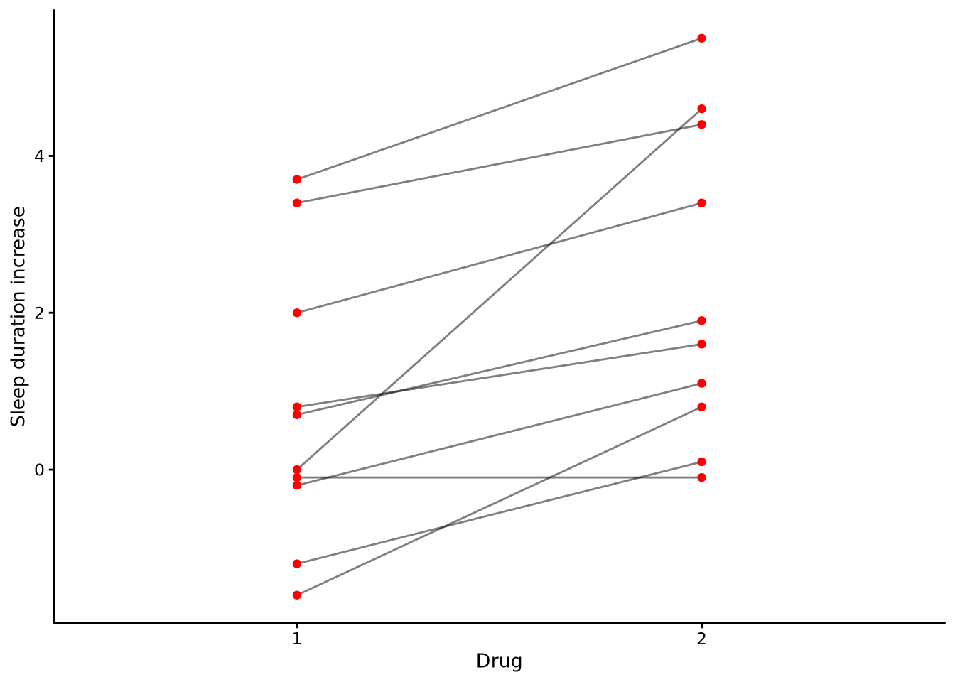
Consider the repeated measures data set from a sleep experiment (shown in long format in Table 10.1 below). This provides the results of an experiment testing the effectiveness of two sleep-inducing drugs. There were 10 participants in the experiment. Each one took two separate drugs on separate occasions and the duration of their sleep relative to a control condition was recorded. For example, for participant 1, their sleep increased by 0.7 hours when they took drug 1 and increased by 1.9 hours when they took drug 2.
Let’s say we are interested in testing whether there is a difference in the average sleep-inducing effects of the two drugs. If this were not repeated measures data and there were two separate groups of 10 participants in each drug condition, then this analysis could be performed using a one-way ANOVA, which in the case of two groups is equivalent to an independent samples t-test, as we have seen in Chapter 7 and Chapter 8. A major assumption of these methods, however, is that the values in each group are sampled independently from normal distributions. Because of this, there should be no correlation between the values in the two groups. This is clearly not the case. There is in fact a correlation of approximately 0.8 between the values in the two drug conditions. The reason for this correlation is due to the fact that the same individuals are being measured on two occasions, and there are individual differences in how either of the sleep-inducing drugs affect people’s sleep. For some people, such as subjects 6 and 7, both drugs have a large effect. For others, such as subjects 2 and 4, both drugs have less of an effect. We can see this phenomenon clearly in Figure 10.1, where we can see that those participants who have higher scores for drug 1 usually have higher scores for drug 2, while those with lower scores on drug 1 usually have lower scores on drug 2 too.
We need to take these correlations into account. We do this by adding a term to the model that represents a person-specific effect, \(\beta_i\). This term accounts for the fact that each person \(i\) contributes data to both conditions meaning their two observations are not independent.
\[ \begin{aligned} y_i &\sim N(\mu_i, \sigma^2), \\ \mu_i &= \beta_0 + \beta_1 \alpha_i + \beta_i \end{aligned} \]
10.2 One-way repeated measures ANOVA
Let us first remind ourselves about how the one-way ANOVA works, and then show how this can be extended to situations where we have repeated measures. As described in Chapter 9, in a one-way ANOVA, we have one outcome or dependent variable and one predictor or independent variable. The dependent variable is a continuous variable, while the independent variable is a categorical variable with \(J\) possible values. As we saw, we can represent our data as a set of \(n\) pairs of values: \[ (y_1, x_1), (y_2, x_2) \ldots (y_n, x_n), \] where \(y_1, y_2 \ldots y_i \ldots y_n\) are all the values of the dependent variable, the \(x_1, x_2 \ldots x_i \ldots x_n\) are the corresponding values of the independent variable, with each value in \(x_1, x_2 \ldots x_n\) having an integer value between \(1\) and \(J\). We said that the one-way ANOVA model assumes that for each \(i\): \[ y_i = \theta + \alpha_{[x_i]} + \epsilon_i, \] where each \(\epsilon_i\) is normally distributed with mean of zero and a standard deviation of \(\sigma\). We said that \(\theta\) is the grand mean and \(\alpha_1, \alpha_2 \ldots \alpha_J\) are the differential effects associated with each of the \(J\) values of the independent variable. The null hypothesis is that \(\alpha_1 = \alpha_2 = \ldots = \alpha_J = 0\). In other words, according to the null hypothesis, the means of the dependent variable corresponding to each value of the independent variable are all the same. We said that we can test this null hypothesis with a model comparison. We set up two alternative models: \[ \begin{aligned} \text{Full model}&\colon y_i = \theta + \alpha_{[x_i]} + \epsilon_i.\\ \text{Restricted model}&\colon y_i = \theta + \epsilon_i. \end{aligned} \] We fit these two models, and then calculate the \(F\) statistic: \[ F = \frac{(\mathrm{RSS}_{R}- \mathrm{RSS}_{F})/(\mathit{df}_{\!R}- \mathit{df}_{\!F})}{\mathrm{RSS}_{F}/\mathit{df}_{\!F}}. \] If the null hypothesis is true, then this statistic will be distributed as a \(F\) distribution with degrees of freedom \(\mathit{df}_{\!R}-\mathit{df}_{\!F}\) and \(\mathit{df}_{\!F}\).
In the one-way repeated measures ANOVA, for each observed value of the outcome variable and independent variable, we also have a new variable that indicates the individual that is being repeatedly measured. In other words, our data can be represented as follows: \[\begin{equation}
(y_1, x_1, s_1), (y_2, x_2, s_2) \ldots (y_n, x_n, s_n),\label{eq:one_within_data}
\end{equation}\] where each \(y_i\) and \(x_i\) are the dependent and independent variables, respectively, and \(s_i\) indicates the identity of individual being measured at observation \(i\). For example, the sleep experiment data is available in R as the built-in dataset sleep, shown in long format in Table 10.1. In this data set, extra is the dependent variable, group is the independent variable, and ID is the variable indicating the individual or subject being repeatedly measured. Using our general terminology, the values of extra in the sleep data set are \(y_1, y_2 \ldots y_n\), the values of group are \(x_1, x_2 \ldots x_n\), and the values of ID are \(s_1, s_2 \ldots s_n\). In this data set, there are only \(K=2\) groups and so each value of the independent variable \(x_i\) takes a value of either \(1\) or \(2\). On the other hand, there are \(J=10\) subjects, so each value of \(s_i\) takes a value from the set \(1, 2 \ldots J=10\).
sleep data set that is built into R, shown in long format which is the required format for repeated measures analyses in R. This data set is a minimal repeated measure data set. We have three variables: extra, group, and ID. These are the dependent, independent, and subject variables, respectively. Each value of the subject variable ID has a value for the dependent variable extra for each of the two values of the independent variable group.
| extra | group | ID |
|---|---|---|
| 0.7 | 1 | 1 |
| -1.6 | 1 | 2 |
| -0.2 | 1 | 3 |
| -1.2 | 1 | 4 |
| -0.1 | 1 | 5 |
| 3.4 | 1 | 6 |
| 3.7 | 1 | 7 |
| 0.8 | 1 | 8 |
| 0.0 | 1 | 9 |
| 2.0 | 1 | 10 |
| 1.9 | 2 | 1 |
| 0.8 | 2 | 2 |
| 1.1 | 2 | 3 |
| 0.1 | 2 | 4 |
| -0.1 | 2 | 5 |
| 4.4 | 2 | 6 |
| 5.5 | 2 | 7 |
| 1.6 | 2 | 8 |
| 4.6 | 2 | 9 |
| 3.4 | 2 | 10 |
The repeated measures one-way ANOVA model extends the original one-way ANOVA model by also using the subject variable. For each \(i\), the repeated measures one-way ANOVA model assumes the following: \[\begin{equation} y_i = \theta + \alpha_{[x_i]} + \phi_{[s_i]} + \epsilon_i.\label{eq:oneway_rmanova} \end{equation}\] Here, just as it did in the case of the original one-way ANOVA, \(\theta\) is the overall mean across all conditions, \(\alpha_{[x_i]}\) represents the effect of the experimental condition for observation \(i\) and \(\epsilon_i\) is the residual error for observation \(i\). In addition, however, we now have \(\phi\) (phi, pronounced “fee”), that is indexed by the subject variable \(s_i\). Given that each \(s_i\) takes a value from \(1\) to \(J\), there are \(J\) values of \(\phi\), i.e. \(\phi_1, \phi_2 \ldots \phi_J\). Each one of these \(J\) values represents the relative effect on the dependent variable of each different subject. For example, if subject \(j\) gets an above average effect from the sleep-inducing drugs, then the value of \(\phi_j\) will be positive; if they experience less improvement \(\phi_j\) will be negative.
Thus far, the one-way repeated measures ANOVA model appears very similar to the two-way ANOVA without an interaction term (see Section 9.3.1). In other words, the dependent variable is determined by the combined effects of two factors plus a random error term representing unexplained variability. However, one important difference between the one-way repeated measures ANOVA and the two-way ANOVA is that the subject-specific factor, i.e. \(\phi_1, \phi_2 \ldots \phi_J\), is assumed to be a random factor, while the independent variable factor \(\alpha_1, \alpha_2 \ldots \alpha_K\) is assumed to be a fixed factor. In other words, each \(\phi_j\) is assumed to be drawn from some probability distribution. In the case of the repeated measures ANOVA, this probability distribution is assumed to be a normal distribution with a mean of zero and standard deviation of \(\tau\). By saying that each \(\alpha_k\) has a fixed value, on the other hand, we are assuming that it has a constant value that is not drawn from a probability distribution.
There are two important consequences of the fact that the subject-specific factor is a random factor. First, this means that the model underlying the repeated measures ANOVA is in fact a type of multilevel model, which we will visit in detail in Chapter 11. In particular, the one-way repeated measures ANOVA model, when it is written in full detail, can be written as follows: \[\begin{equation} \begin{aligned} y_i &= \theta + \alpha_{[x_i]} + \phi_{[s_i]} + \epsilon_i, \quad \epsilon_i \sim N(0, \sigma^2) \quad \text{for $i \in 1 \ldots n$},\\ \phi_j &\sim N(0, \tau^2),\quad \text{for $j \in 1 \ldots J$}. \end{aligned} \end{equation}\] This is effectively a varying intercept multilevel model of the kind seen in Chapter 11, e.g. Section 11.3.
A second consequence of the fact that the subject-specific factor is a random factor is that this can affect how we calculate the denominator term in F statistics to test null hypotheses. In other words, were we to test the null hypothesis about the repeated measures factor in a repeated measures ANOVA, the denominator term for the F statistic will not necessarily be calculated the same way as it would if there were only fixed factors, as is the case with non-repeated measures ANOVA. We will see examples of these different calculations in later sections.
10.2.1 Null hypothesis testing
In the one-way repeated measures ANOVA, we test the null hypothesis about the effect of the independent variable. Just as we have seen in the ANOVA analyses in Chapter 9, this is the hypothesis that in the population, the average value of the dependent variable is the same for each value of the independent variable. This is equivalent to the following hypothesis: \[ H_0 \colon \alpha_1 = \alpha_2 \ldots = \ldots \alpha_K = 0. \] We can test this hypothesis by, as we have done repeatedly, considering two alternative models: \[ \begin{aligned} \text{Full model}&\colon y_i = \theta + \alpha_{[x_i]} + \phi_{[s_i]} + \epsilon_i.\\ \text{Restricted model}&\colon y_i = \theta + \phi_{[s_i]} + \epsilon_i. \end{aligned} \]
These two models differ by the presence of the \(\alpha_{[x_i]}\) term of the full model and its absence in the restricted model and so the null hypothesis that \(\alpha_1 = \alpha_2 \ldots = \ldots \alpha_K = 0\) is true if and only if these two models are identical. Just as before, we fit these two models and then calculate the \(F\) statistic \[ F = \frac{(\mathrm{RSS}_{R}- \mathrm{RSS}_{F})/(\mathit{df}_{\!R}- \mathit{df}_{\!F})}{\mathrm{RSS}_{F}/\mathit{df}_{\!F}}, \] which is distributed as a \(F\)-distribution with degrees of freedom \(\mathit{df}_{\!R}- \mathit{df}_{\!F}\) and \(\mathit{df}_{\!F}\) if the null hypothesis is true.
There are very many ways to perform this analysis in R. Here, we will use the aov_car() function from the sgsur (reexported from the afex (Analysis of Factorial EXperiments) package).
Using the sleep data set and testing the null hypothesis that there is no effect of the independent variable group, the required aov_car() command is as follows:
M_10_1 <- aov_car(extra ~ Error(ID/group), data = sleep)Before we look at the results, let us discuss the syntax that we have used here. The extra ~ is the familiar way we specify the outcome or dependent variable of an analysis. The Error(...) term is new, however. This is used to specify the subject indicator variable and any within-subjects variables. A within-subjects variable is any independent variable such that for each subject, the dependent variable is measured at each level of that variable. In this analysis, the group variable is a within-subjects variable because for each subject, the dependent variable is measured at each level of group. Thus, by Error(ID/group), we are saying that ID is the random factor subject variable and that group is a within-subject variable. Even if the Error(ID/group) does not feel very clear and intuitive yet, it is likely to become clearer with some further examples, which we will see below.
We could write this sample model using the formula extra ~ group + Error(ID/group) instead of extra ~ Error(ID/group). It is not uncommon to see this kind of formula for aov_car()-based repeated measures ANOVA. However, these two models are identical. In the help page for aov_car, see help(aov_car), it states the following: “Factors outside the Error term are treated as between-subject factors (the within-subject factors specified in the Error term are ignored outside the Error term; in other words, it is not necessary to specify them outside the Error term …)”.
Now, let us look at the results, which we do using the generic summary function.
summary(M_10_1)
Univariate Type III Repeated-Measures ANOVA Assuming Sphericity

            Sum Sq num Df Error SS den Df F value   Pr(>F)
(Intercept) 47.432      1   58.078      9  7.3503 0.023953 *
group       12.482      1    6.808      9 16.5009 0.002833 **
---
Signif. codes:  0 '***' 0.001 '**' 0.01 '*' 0.05 '.' 0.1 ' ' 1
The (Intercept) row in the ANOVA table is of no relevance and can be ignored. It just tests a null hypothesis about the intercept term. The group row, on the other hand, provides all the terms in the right-hand side of the \(F\) statistic:
Sum Sq= \((\mathrm{RSS}_{R}- \mathrm{RSS}_{F}) = 12.482\)num Df= \((\mathit{df}_{\!R}- \mathit{df}_{\!F}) = 1\)Error SS= \(\mathrm{RSS}_{F}= 6.808\)den Df= \(\mathit{df}_{\!F}= 9\)
The value of F value = \(16.5009\) is therefore obtained as follows: \[
F = \frac{(\mathrm{RSS}_{R}- \mathrm{RSS}_{F})/(\mathit{df}_{\!R}- \mathit{df}_{\!F})}{\mathrm{RSS}_{F}/\mathit{df}_{\!F}}= \frac{
12.482/1
}{
6.808/9
} = 16.5009.
\] The p-value, displayed as Pr(>F), of 0.002833 is the probability of getting a value as large or larger than \(16.5009\) in an F distribution whose degrees of freedom are 1 and 9.
We can also obtain the main results, with some of the unnecessary details presented above omitted, by simply typing the name of the model M_10_1, or equivalently by typing nice(M_10_1):
M_10_1Anova Table (Type 3 tests)
Response: extra
Effect df MSE F ges p.value
1 group 1, 9 0.76 16.50 ** .161 .003
---
Signif. codes: 0 '***' 0.001 '**' 0.01 '*' 0.05 '+' 0.1 ' ' 1From this, we obtain the rounded \(F\) statistic, the two degrees of freedom, and the rounded p-value. It also displays MSE, which is simply 6.808/9. It also displays ges, which stands for generalised eta squared, and is usually written \(\eta_{G}^2\). This is a recommended effect size for repeated measures analysis (Bakeman, 2005). We will return to effect sizes and \(\eta_{G}^2\) below. As usual, we would write this ANOVA result in summary form as follows: \(F(1, 9) = 16.501\), \(p = 0.003\), \(\eta_{G}^2= 0.161\).
The ANOVA just tests a null hypothesis. From the result just reported, we now know that the null hypothesis that there is no difference in the average effects of the two drugs can be rejected, but it is rare that we are interested in this result alone. At the very least, we are usually also interested in knowing the average effects of each drug. As we have seen above, we can obtain these effects by calculating estimated marginal means, which can be done using the emmeans() function:
M_10_1_emm <- emmeans(M_10_1, ~ group)
M_10_1_emm
group emmean SE df lower.CL upper.CL
X1 0.75 0.566 9 -0.530 2.03
X2 2.33 0.633 9 0.898 3.76
Confidence level used: 0.95 Although we already know that these two means are significantly different, we can also obtain that result by doing a post-hoc comparison of means using the pairs command from emmeans:
pairs(emmeans(M_10_1, ~group)) contrast estimate SE df t.ratio p.value
X1 - X2 -1.58 0.389 9 -4.062 0.0028Note how the p-value for this result is identical to that of the ANOVA’s \(F\) test. In fact, the ANOVA’s \(F\) statistic is exactly the square of this post-hoc comparison’s \(t\) statistic. Whenever there are just two levels of the within-subject variable in the one-way repeated measures ANOVA, this will always be the case.
10.2.2 Sphericity
The validity of the repeated measures ANOVA is based on assumptions, many of which are identical to those of non-repeated measures ANOVA. For example, it is assumed that the residuals are independent and normally distributed with a mean of zero. In addition, however, repeated measures ANOVA makes a strong assumption known as the sphericity assumption. This is an important matter in repeated measures ANOVA because when this assumption is not met, and in fact it is often not met in practice, the \(F\) statistic for the null hypothesis test does not follow an \(F\) distribution and the reported p-values will be lower than their true values, thus leading to an increased Type I error rate. Fortunately, when the assumption is not met, we can apply adjustments to the \(F\) tests to more accurately calculate the correct p-values. In this section, we will describe the sphericity assumption and these corrections.
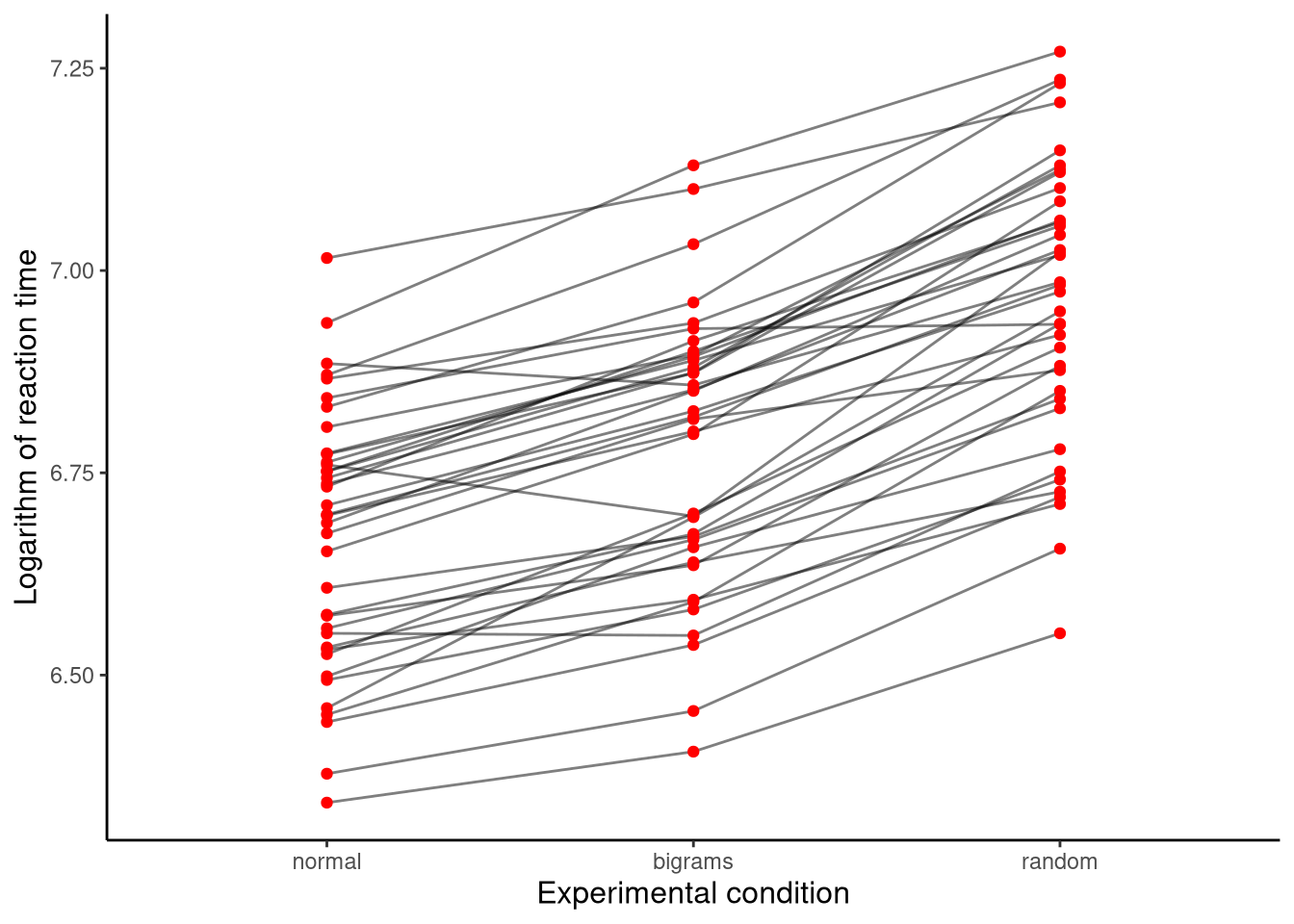
As we will see below, the sphericity assumption is necessarily met if we only have two levels to the within-subjects variable, as we did in the case of the sleep analysis. In order to properly explore this assumption, therefore, we need to consider analyses where the within-subject variable has three or more levels. As an example, consider the data shown in Figure 10.2. This data, taken from Behmer (2017), shows the average keyboard typing times of each of 38 subjects in each of three different experimental conditions: the “normal” condition where subjects typed English words, the “bigram” condition where subjects typed non-words that contained typical English bigrams (i.e., consecutive letter pairs), and the “random” condition where subjects typed non-words consisting of random letters. A major question of interest may be whether the average response time differs across the three experimental conditions. We can address this with a one-way repeated measures ANOVA.
Note 10.1: Covariance Matrices and Sphericity
A covariance matrix gives covariances (correlation times product of standard deviations) between pairs of variables. If sphericity holds in a \(k \times k\) covariance matrix \(\Sigma\), each element \(\Sigma_{ij}\) satisfies \(\Sigma_{ij} = a_i + a_j + \lambda \delta_{ij}\), where \(a_1, \ldots, a_k\) is a vector, \(\lambda\) is constant, and \(\delta_{ij} = 1\) if \(i=j\), else \(0\) (Huynh, 1970).
The sphericity assumption can be stated in different but equivalent ways. Most directly, it is defined in terms of the properties of the covariance matrix of the effects of the within-subject variable (see Note 10.1). An equivalent definition, but one that is much easier to understand, is in terms of homogeneity of the variance of difference scores of the within-subjects variable. This is similar to the homogeneity of variance assumption in the non-repeated measures ANOVA that required that the variance of the dependent variable be the same for each level of the independent variable. In the repeated measures ANOVA, the homogeneity of the difference variances requires the variances of the differences of each pair of levels of the within-subjects variable to be the same. We can now see why sphericity necessarily holds whenever there are just two levels to the within-subjects variable: if there are only two levels, there is only one possible difference of levels.
It should be emphasised that the sphericity assumption is an assumption about the population, not the sample. In any one sample, even if sphericity holds in the population, we may not observe homogeneity of the variances of differences between levels due to sampling variation. Nonetheless, to understand this assumption, it is helpful to consider that if sphericity is correct, the variances of the differences between each pair of levels of the within-subjects variable should be approximately equal.
If the assumption of sphericity is not met, the immediate consequence is that the degrees of freedom for the ANOVA’s \(F\) distribution are too large. More precisely, if the sphericity assumption is violated, the sampling distribution of the \(F\) statistic is approximately that of an \(F\) distribution whose degrees of freedom are lower than those calculated using the usual ANOVA rules, i.e. \(\mathit{df}_{\!R}- \mathit{df}_{\!F}\) and \(\mathit{df}_{\!F}\) in the one-way case. If the degrees of freedom are overstated, then the resulting p-values are necessarily understated; the true p-value is higher than the one reported. Our way of resolving this problem is to adjust the degrees of freedom downwards. Note 10.2 showed that if we knew the true nature of the statistical population, we could calculate a quantity named \(\epsilon\) that takes values between \(1/(k - 1)\) and \(1\), where \(k\) is the number of levels of the within-subjects variable, and then adjust the degrees of freedom by multiplying them by \(\epsilon\). If the sphericity assumption is met, then \(\epsilon =1\), and there is no adjustment to the degrees of freedom. On the other hand, the greater the violation of the sphericity assumption, the lower the value of \(\epsilon\) is, and so the greater the downward adjustment of the degrees of freedom. Of course, because we never know the properties of the population, we cannot calculate \(\epsilon\). However, Greenhouse & Geisser (Geisser, 1958; Greenhouse & Geisser, 1959) estimated the value of \(\epsilon\) using the sample data itself (see Note 10.2) and named their estimator \(\hat{\epsilon}\) (pronounced epsilon-hat). The degrees of freedom of the \(F\) distribution are then adjusted by multiplying by \(\hat{\epsilon}\). This is known as the Greenhouse-Geisser correction.
Note 10.2: Sphericity correction factors
Greenhouse & Geisser’s \(\hat{\epsilon}\) is calculated from the sample covariance matrix \(S\) (Geisser, 1958; Greenhouse & Geisser, 1959). An alternative, \(\tilde{\epsilon}\) (Huynh & Feldt, 1976), modifies \(\hat{\epsilon}\) based on sample size \(n\). For large \(n\), both give similar values. Following Maxwell et al. (2017) (p. 634), we use \(\hat{\epsilon}\) as default since \(\tilde{\epsilon}\) can increase Type I error rates.
Let us now perform a one-way repeated measures ANOVA on the Behmer (2017) typing data where we analyse whether there is a difference in the average typing speed across the three conditions. The relevant data is available from the sgsur package by the name behmercrump_vis. The following command performs the analysis.
M_10_2 <- aov_car(log_rt ~ Error(subject/condition), data = behmercrump_vis)Note that the syntax is identical to that used for model M_10_1 for the sleep data above. Within the Error term, we indicate the subject indicator variable subject and the within-subjects variable condition. Let us now look at the summary output of this analysis.
summary(M_10_2)
Univariate Type III Repeated-Measures ANOVA Assuming Sphericity

            Sum Sq num Df Error SS den Df  F value    Pr(>F)
(Intercept) 5275.6      1  2.96868     37 65752.32 < 2.2e-16 ***
condition      1.6      2  0.19109     74   312.87 < 2.2e-16 ***
---
Signif. codes:  0 '***' 0.001 '**' 0.01 '*' 0.05 '.' 0.1 ' ' 1


Mauchly Tests for Sphericity

          Test statistic   p-value
condition        0.75209 0.0059276


Greenhouse-Geisser and Huynh-Feldt Corrections
 for Departure from Sphericity

           GG eps Pr(>F[GG])
condition 0.80134  < 2.2e-16 ***
---
Signif. codes:  0 '***' 0.001 '**' 0.01 '*' 0.05 '.' 0.1 ' ' 1

             HF eps   Pr(>F[HF])
condition 0.8320114 4.646372e-31
Clearly, there is a lot more information here than was the case for the M_10_1 analysis. The reason for this is simply because in this analysis, the within-subjects variable condition has three levels, while in M_10_1, the within-subjects variable group had only two levels. As mentioned above, the sphericity assumption is necessarily met whenever there are two levels, but when there are three or more levels to the within-subjects variable, the assumption of sphericity will not necessarily be met. All the extra information in the M_10_2 summary output compared to that of M_10_1 concerns the sphericity assumption. Let us now go through all this extra information.
First, there is a section named Mauchly Tests for Sphericity. This is the result of Mauchley’s sphericity test (Mauchly, 1940). This is a traditional hypothesis test that tests the null hypothesis that the assumption of sphericity is true: if its p-value is low, then the assumption of sphericity can be rejected. While Mauchly’s test has a long tradition of use in repeated measures ANOVA and is still widely used, it is not a very useful test. It is prone to high Type II error rates, especially with small sample sizes and when the data is not normal, which means that the assumption of sphericity is often not rejected even when it is false (Cornell & Berger, 1992; see Keselman, 1980). Following Maxwell et al. (2017), pp. 629-630, we don’t recommend using Mauchly’s test and prefer to always use the Greenhouse & Geisser \(\hat{\epsilon}\) adjustment. As we will see, this is also the default behaviour of aov_car.
Next, we see the value of Greenhouse & Geisser’s \(\hat{\epsilon}\) sphericity correction factor, whose value is \(\hat{\epsilon} = 0.80134\). As explained above, this value is multiplied by the ANOVA’s \(F\) distribution’s degrees of freedom, which are 2 and 74, as we can see in the condition row of the ANOVA table above. By multiplying by 0.80134, these will be adjusted down to 1.6 and 59.3, respectively. The p-value for the \(F\) test using these adjusted degrees of freedom is the corresponding value under the label Pr(>F[GG]).
Finally, we see the value of the Huynh & Feldt \(\tilde{\epsilon}\) sphericity correction factor (see Note 10.2) whose value is \(\tilde{\epsilon} = 0.83201\). This is an alternative adjustment factor to the Greenhouse & Geisser \(\hat{\epsilon}\) factor, but we will not consider it further here, preferring to always use \(\hat{\epsilon}\), which is also the default behaviour of aov_car, as we will see.
Having reviewed all the information in the summary output, our primary interest lies in just two lines: the condition row of the ANOVA table, and the value of \(\hat{\epsilon}\). Moreover, to obtain the adjusted degrees of freedom, we would need to manually multiply the degrees of freedom in the condition row by \(\hat{\epsilon}\). Fortunately, by simply typing the name M_10_2, or equivalently typing nice(M_10_2), we get all and only this information in a very useful and compact form:
M_10_2Anova Table (Type 3 tests)
Response: log_rt
Effect df MSE F ges p.value
1 condition 1.60, 59.30 0.00 312.87 *** .338 <.001
---
Signif. codes: 0 '***' 0.001 '**' 0.01 '*' 0.05 '+' 0.1 ' ' 1
Sphericity correction method: GG The ANOVA table is now presented in compact form, omitting the irrelevant information about the intercept term. Under df, we have 1.60, 59.30. These are the adjusted degrees of freedom obtained by multiplying, as we just saw, the original degrees of freedom of 2 and 74 by 0.80134. We also know that the adjustment is obtained by multiplying by \(\hat{\epsilon} = 0.80134\), and not by the Huynh-Feldt factor \(\tilde{\epsilon} = 0.83201\), because the correction method is stated at the bottom as GG (Greenhouse-Geisser). Under F, we have 312.87 ***. Obviously, the value of the \(F\) statistic itself is 312.87, while the *** gives the significance code, as described underneath. Next, we have the \(\eta_{G}^2\) value of 0.338. Finally, there is the p-value, expressed as an inequality as its value is less than 0.001. Given that the p-value is extremely low, we reject the null hypothesis that there is no difference in the effect of the condition independent variable on the log_rt dependent variable. If we were communicating these results in a report or paper, the main results would be stated as follows: \(F(1.6, 59.3) = 312.87\), \(p < 0.001\), \(\hat{\epsilon} = 0.801\), \(\eta_{G}^2= 0.338\).
As usual, we are interested in more than just the results of the null hypothesis test. We are also interested in the estimated marginal means of the effects of each condition, which we can obtain from the emmeans command:
M_10_2_emm <- emmeans(M_10_2, ~ condition)
M_10_2_emm
condition emmean SE df lower.CL upper.CL
normal 6.67 0.0262 37 6.62 6.72
bigrams 6.78 0.0276 37 6.72 6.83
random 6.96 0.0283 37 6.90 7.02
Confidence level used: 0.95 Note that the confidence intervals are very tight around the estimated means. Each confidence interval is roughly twice the standard error, which is very small relative to the size of the effect. We can do a post-hoc comparison of all pairs of effects, which adjusts the p-values using Tukey’s range test, using the pairs command:
pairs(M_10_2_emm) contrast estimate SE df t.ratio p.value
normal - bigrams -0.108 0.00931 37 -11.565 <0.0001
normal - random -0.289 0.01420 37 -20.365 <0.0001
bigrams - random -0.181 0.01100 37 -16.492 <0.0001
P value adjustment: tukey method for comparing a family of 3 estimates Finally, we can plot these effects and confidence intervals, including showing arrows to indicate if the effects are significantly different, by passing the M_10_2_emm object to plot, with the result shown in Figure 10.3:
plot(M_10_2_emm, horizontal = F, comparisons = TRUE) + theme_classic()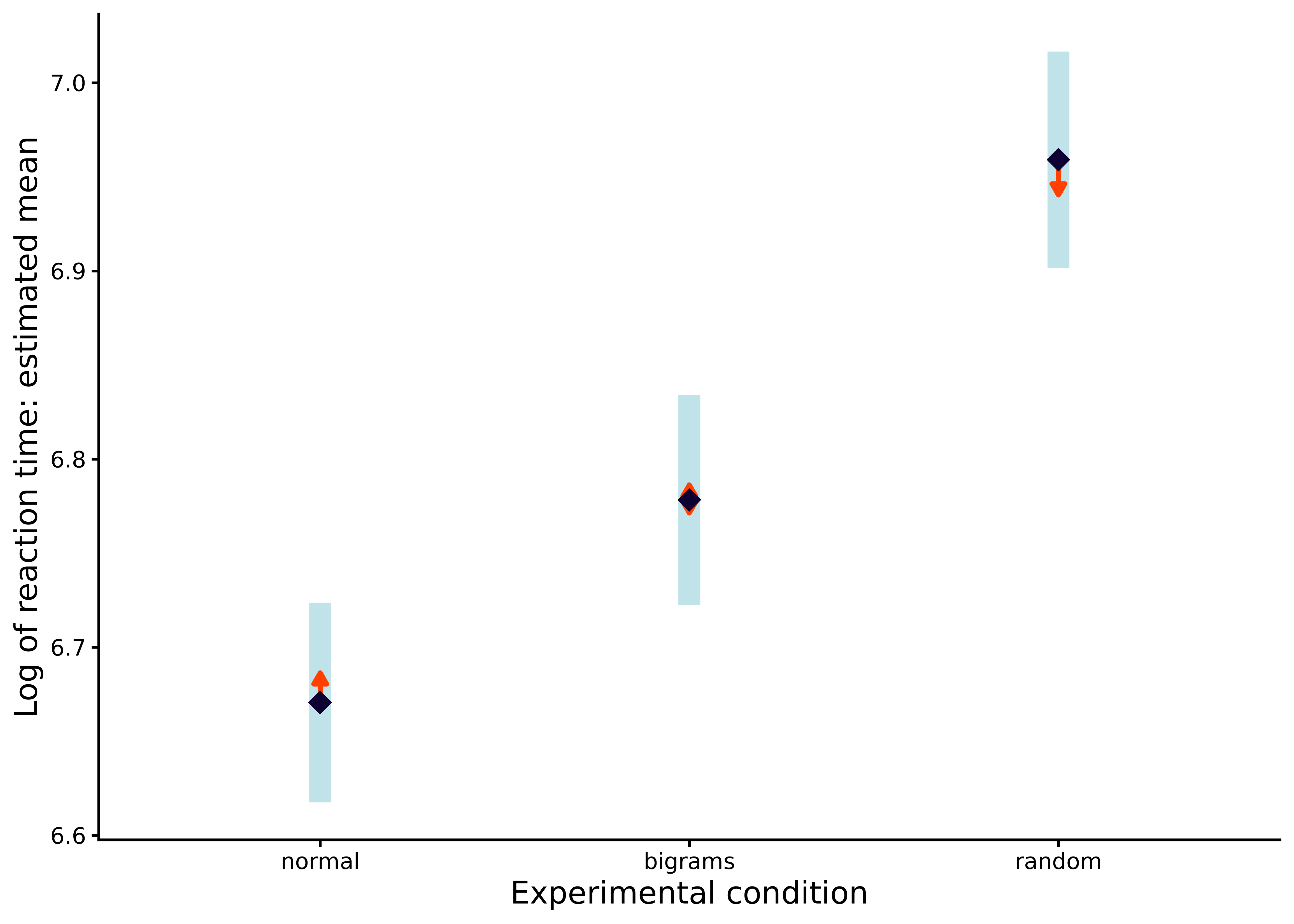
10.3 Two-way repeated measures ANOVA
In this section, we will consider factorial repeated measures ANOVA, albeit restricting ourselves to problems with just two independent variables. Although repeated measures ANOVA with three or more factors are common in practice, the concepts and practices covered here can be relatively easily extended to these cases. In any two-way repeated measures ANOVA, there must be at least one within-subjects variable. The second independent variable may be another within-subjects variable. In this case, which we will refer to as a two within-subjects repeated measures ANOVA, each subject is measured on the dependent variable at each possible combination of the two independent variables. It is possible, however, for the second independent to be a between-subjects variable. In other words, each subject is measured on the outcome variable at one and only one level of one independent variable, which is the between-subjects variable, but at all levels of the other independent variable, the within-subjects variable. This type of ANOVA is sometimes referred to as a one-within one-between repeated measures ANOVA. It is also sometimes known as mixed design repeated measures ANOVA. However, it is important to note that the term “mixed” is used in distinct senses in repeated measures analyses, and so it is important not to confuse these senses. These designs are also known as split-plot designs, which is a term that originated in agricultural science where fields (the “plots”) were divided into separate groups and then each sub-divided into sub-plots (the “splits”).
10.3.1 Two within-subjects factors
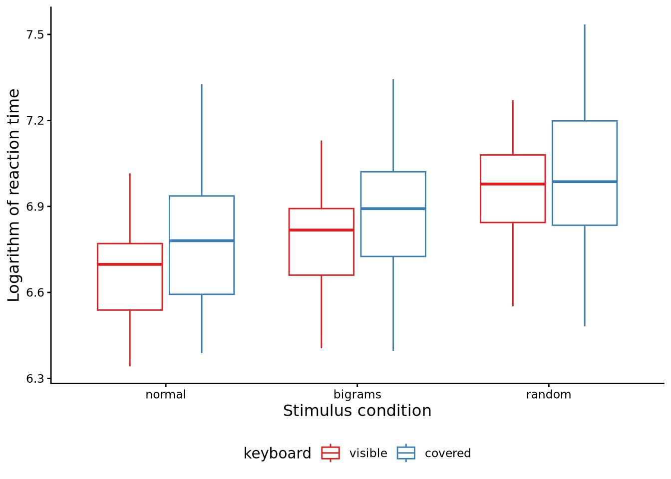
Consider the data shown in Figure 10.4. The data, like that used above, is from the Behmer (2017) study. As we saw above, in that study, subjects had their key typing response times recorded for each of three different types of letter stimuli (i.e. “normal”, “bigrams”, and “random”). In addition, however, each subject did this typing under two different keyboard conditions: either they saw the keyboard as normal or else the keyboard was covered. Previously, we had just used the data from the keyboard visible condition. This data set is available in sgsur by the name behmercrump_vis. The data set that provides both keyboard conditions is also in sgsur, by the name behmercrump. Figure 10.4 shows the boxplots in each combination of the two independent variables, making the average effects of both independent variables apparent.
In a two-way repeated measures ANOVA, we can represent the data as follows: \[
(y_1, x_1, z_1, s_1), (y_2, x_2, z_2, s_2), \ldots (y_n, x_n, z_n, s_n).
\] This is an extension of the form of the data for the one within-subjects case. Again, each \(y_i\) and \(s_i\) are the dependent variable and the subject indexing variable, respectively, at observation \(i\). Likewise, each \(x_i\) is an independent variable at observation \(i\). The new variable, \(z_i\), represents the second independent variable. The two independent variables and the subject variable are all categorical variables. Following the same notation we use above for the one-way case, we say that each \(x_i\) takes on values from the set \(1\ldots K\), and \(s_i\) takes values from the set \(1 \ldots J\). In other words, there are \(K\) levels to the first independent variable, and there are \(J\) subjects. For the second independent variable, \(z_i\), we will say that it has \(L\) levels so takes values from the set \(1 \ldots L\). There are \(n = 228\) observations in total, so the data set can be represented as an \(n\) by \(4\) dataframe in R. Using our terminology, on row \(i\), \(y_i\) represents the value of log_rt, \(s_i\) represents the value of subject, \(x_i\) represents the value of condition, and \(z_i\) represents the value of keyboard. Given that there are 3 levels to the condition variable, 2 levels to the keyboard variable, and 38 subjects, in this data, we have \(K = 3\), \(L = 2\), and \(J = 38\).
The underlying statistical model in a two within-subjects repeated measures ANOVA has considerably more terms than the one-way case. For each \(i\), this new two-way ANOVA is as follows: \[\begin{equation} y_i = \theta + \alpha_{[x_i]} + \beta_{[z_i]} + (\alpha\beta)_{[x_i, z_i]} + (\alpha\phi)_{[x_i,s_i]} + (\beta\phi)_{[z_i,s_i]} + \phi_{[s_i]} + \epsilon_{i}.\label{eq:twowithin_rmanova} \end{equation}\] Compared to the one-way case, there are three new terms: \((\alpha\beta)_{[x_i, z_i]}\), \((\alpha\phi)_{[x_i,s_i]}\), and \((\beta\phi)_{[z_i,s_i]}\). The \((\alpha\beta)_{[x_i, z_i]}\) is the interaction term, just like in the case of the two-way ANOVA we considered in Section 9.3. This term allows us to model how the effect of the two independent variables on the dependent variable is more than just the sums of its parts. By analogy, \((\alpha\phi)_{[x_i,s_i]}\), and \((\beta\phi)_{[z_i,s_i]}\) are interaction terms for the interactions with each of the two independent variables and the subject variable. These allow us to model how the effects of each independent variable vary across subjects. In other words, for example, the effect of each independent variable is allowed to vary from subject to subject and is not a constant for each subject. Note that we do not have a three-way interaction term, \((\alpha\beta\phi)_{[x_i,z_i,s_i]}\). In principle, this term is possible but only in the case where we have multiple observations for each subject in each combination of the two independent variables. Otherwise, it is not possible to identify the three-way interaction term. In general, any term indexed by the subject index \(s_i\) is a random factor. In the one-way repeated measures case, there was just one such term, namely \(\phi_{[s_i]}\). In this two within-subjects analysis, there are three such terms. Each one is assumed to be random in the sense that it is drawn from some probability distribution, specifically a normal distribution. More immediately, the fact that these variables are random affects the denominator of the F tests that we use to test the effects of the independent variables and their interaction.
Although there are many terms in the model, the standard focus is on just three of these terms. This is because it addresses three separate null hypotheses: \[ \begin{aligned} H^{\alpha}_0 &\colon \alpha_1 = \alpha_2 = \ldots \alpha_K = 0,\\ H^{\beta}_0 &\colon \beta_1 = \beta_2 = \ldots \beta_L = 0,\\ H^{\alpha\beta}_0 &\colon \alpha\beta_{1,1} = \alpha\beta_{1,2} = \ldots \alpha\beta_{LK} = 0. \end{aligned} \] To test these hypotheses, we compare the three following restricted models to the full model: \[ \begin{aligned} \text{Restricted model}^\alpha&\colon y_i = \theta + \beta_{[z_i]} + (\alpha\beta)_{[x_i, z_i]} + (\alpha\phi)_{[x_i,s_i]} + (\beta\phi)_{[z_i,s_i]} + \phi_{[s_i]} + \epsilon_{i},\\ \text{Restricted model}^\beta&\colon y_i = \theta + \alpha_{[x_i]} + (\alpha\beta)_{[x_i, z_i]} + (\alpha\phi)_{[x_i,s_i]} + (\beta\phi)_{[z_i,s_i]} + \phi_{[s_i]} + \epsilon_{i},\\ \text{Restricted model}^{\alpha\beta}&\colon y_i = \theta + \alpha_{[x_i]} + \beta_{[z_i]} + (\alpha\phi)_{[x_i,s_i]} + (\beta\phi)_{[z_i,s_i]} + \phi_{[s_i]} + \epsilon_{i}. \end{aligned} \] As can be seen, each restricted model is equal to the full model but when the corresponding null hypothesis is true. In other words, for example, if \(H^\alpha\) is true in the full model, then this is identical to Restricted model\(^\alpha\).
To test these hypotheses, as per usual, we fit these models and then for each restricted model, calculate an \(F\) statistic that will be distributed as an \(F\) distribution if its corresponding null hypothesis is true. There is one complication here, however. As mentioned, the fact that some of the factors in these models are random factors affects the denominator term in the \(F\) statistics. In other words, while the numerator of the \(F\) statistic will be formed in the usual manner, the denominator will not necessarily be \(\mathrm{RSS}_{F}/\mathit{df}_{\!F}\). Instead, for each restricted model, the denominator will have its own denominator term. This also leads to a different second degree of freedom term for the \(F\) statistic. Specifically, the two degrees of freedom for the \(F\) statistics for \(H^\alpha_0\), \(H^\beta_0\), and \(H^{\alpha\beta}_0\) are as follows: \[ \begin{aligned} H^{\alpha}_0 &\colon K-1, (K-1)(J-1) ,\\ H^{\beta}_0 &\colon L-1, (L-1)(J-1),\\ H^{\alpha\beta}_0 &\colon (K-1)(L-1), (K-1)(L-1)(J-1). \end{aligned} \]
10.3.1.1 Two within-subjects ANOVA using R
To perform a two within-subjects ANOVA using the behmercrump data set, we will use aov_car as we did with the one-way repeated measures ANOVA. Inside the Error term, we indicate the subject index variable and also the two within-subject variables. For the present analysis, this is done as follows:
M_10_3 <- aov_car(log_rt ~ Error(subject/condition * keyboard), data = behmercrump)Notice that within the Error term, we have condition * keyboard to the right of subject/. This is how we specify that both condition and keyboard are within-subject variables and also that we want to address the main effects of both of these variables and their interaction. Had we wished to not model the interaction, we would have written condition + keyboard as opposed to condition * keyboard.
Let us first examine the results provided by the summary command:
summary(M_10_3)
Univariate Type III Repeated-Measures ANOVA Assuming Sphericity

                    Sum Sq num Df Error SS den Df   F value    Pr(>F)
(Intercept)        10672.5      1   7.8900     37 50048.240 < 2.2e-16 ***
condition              2.3      2   0.4266     74   200.635 < 2.2e-16 ***
keyboard               0.3      1   0.9425     37    13.600 0.0007224 ***
condition:keyboard     0.1      2   0.2785     74    11.474 4.568e-05 ***
---
Signif. codes:  0 '***' 0.001 '**' 0.01 '*' 0.05 '.' 0.1 ' ' 1


Mauchly Tests for Sphericity

                   Test statistic p-value
condition                 0.67197 0.00078
condition:keyboard        0.96161 0.49429


Greenhouse-Geisser and Huynh-Feldt Corrections
 for Departure from Sphericity

                    GG eps Pr(>F[GG])
condition          0.75300  < 2.2e-16 ***
condition:keyboard 0.96303  5.952e-05 ***
---
Signif. codes:  0 '***' 0.001 '**' 0.01 '*' 0.05 '.' 0.1 ' ' 1

                      HF eps   Pr(>F[HF])
condition          0.7779875 2.315597e-24
condition:keyboard 1.0148590 4.567985e-05
As we saw above for model M_10_2, this summary output can be quite detailed, with an ANOVA table, the results of the Mauchly test, and the sphericity correction factors and their p-value adjustments using both the Greenhouse-Geisser and Huynh-Feldt methods. Let us go through each of these in turn.
The ANOVA table contains four rows. We can ignore the first row, labelled (Intercept), as this provides the results of an \(F\) test testing the null hypothesis that \(\theta = 0\). It is highly unlikely that this hypothesis is ever of real interest. On the other hand, the remaining three rows provide the \(F\) test results for the null hypothesis tests of \(H^\alpha_0\), \(H^\beta_0\), and \(H^{\alpha\beta}_0\), respectively, albeit using the original degrees of freedom and p-values that are as yet unadjusted for sphericity violations. We will see these adjustments applied momentarily. Each row provides the \(F\) test’s numerator and denominator sums of squares, listed as Sum Sq and Error Sq, respectively, and the unadjusted numerator and denominator degrees of freedom, listed as num Df and den Df, respectively, and the resulting \(F\) statistics, listed as F value, and the resulting unadjusted p-value, listed as Pr(>F). For example, the \(F\) statistic for the \(H^\alpha_0\) null hypothesis, is obtained as follows: \[
F = \frac{2.3/2}{0.4266/74},
\] which has the stated F value of \(200.635\) when calculated with full decimal precision.
Although we will adjust the degrees of freedom to take into account sphericity corrections, it is useful to review their unadjusted values with respect to the rules for the calculation of degrees of freedom that we mentioned previously. Using the fact that \(K = 3\), \(L = 2\), and \(J = 38\), applying the rules above, we get the following degrees of freedom pairs for each hypothesis: \[ \begin{aligned} H^{\alpha}_0 &\colon K-1, (K-1)(J-1) = 2, 74,\\ H^{\beta}_0 &\colon L-1, (L-1)(J-1) = 1, 37,\\ H^{\alpha\beta}_0 &\colon (K-1)(L-1), (K-1)(L-1)(J-1) &= 2, 74. \end{aligned} \] We see that these match the numerator and denominator degrees of freedom in the ANOVA table.
Next in the summary output is the results of the Mauchly test of sphericity. We see a low p-value for the sphericity corresponding to the condition variable, a high p-value for that corresponding to the interaction. Note that there is no result for the keyboard. This is because, as we have seen, the sphericity condition is necessarily met if there are only two levels of the repeated measures factor. This means that according to Mauchly’s test, sphericity is being violated for the condition variable but not for the interaction. However, as mentioned above, Mauchly’s test has limited usefulness given that we will always apply the sphericity correction factors. Knowing the results of Mauchly’s test may give us a sense of how much correction will be applied — relatively little if any for the interaction, but a greater one for the condition variable — but it is also susceptible to Type II errors (i.e., missing sphericity violations), and in some cases, even very low p-values may correspond to relatively minimal sphericity corrections. For this reason, and following Keselman (1980), Cornell & Berger (1992), Maxwell et al. (2017), the results of Mauchly’s test are not particularly valuable.
Next, we see the Greenhouse-Geisser \(\hat{\epsilon}\) and the Huyhn-Feldt \(\tilde{\epsilon}\) sphericity correction factors for the condition and the condition:keyboard interaction. Note that from each method we get a separate correction factor for each factor or interaction. These are then multiplied by the appropriate degrees for each \(F\) test. Also note that \(\hat{\epsilon}\) and \(\tilde{\epsilon}\) are relatively similar for each effect. As we mentioned above, however, we will default to using the Greenhouse-Geisser \(\hat{\epsilon}\) because the Huyhn-Feldt \(\tilde{\epsilon}\) may lead to a slight increase in Type I error. Also note that for the interaction, \(\tilde{\epsilon}\) is greater than \(1.0\). This is essentially an error due to the method of estimation because the true value of the \(\epsilon\) population variable being estimated has \(\epsilon=1\) as its upper bound. In situations like this where the estimator is greater than \(1\), it is rounded down to \(1.0\) when it is applied as the correction factor. Finally, the p-values that will occur once the \(\hat{\epsilon}\) or \(\tilde{\epsilon}\) corrections are applied are also shown under Pr(>F[GG]) and Pr(>[HF]), respectively.
Although the details provided by the summary command are useful in order to appreciate more details of the analysis, the vital information can be displayed in a succinct manner just by typing the name of the model, or equivalently by using the nice command:
M_10_3Anova Table (Type 3 tests)
Response: log_rt
Effect df MSE F ges p.value
1 condition 1.51, 55.72 0.01 200.63 *** .195 <.001
2 keyboard 1, 37 0.03 13.60 *** .035 <.001
3 condition:keyboard 1.93, 71.26 0.00 11.47 *** .009 <.001
---
Signif. codes: 0 '***' 0.001 '**' 0.01 '*' 0.05 '+' 0.1 ' ' 1
Sphericity correction method: GG In this output, as can be easily verified, the values of \(\hat{\epsilon}\) for condition and the condition:keyboard interaction are multiplied by the appropriate degrees of freedom. The p-values are then obtained by calculating the probability of a value greater than the \(F\) statistic in an \(F\) distribution with the adjusted degrees of freedom. Clearly, for all three null hypotheses being tested, the corresponding p-values are very low, which means that there is negligible evidence in favour of each of the three hypotheses being tested, namely \[
\begin{aligned}
H^{\alpha}_0 &\colon \alpha_1 = \alpha_2 = \ldots \alpha_K = 0,\\
H^{\beta}_0 &\colon \beta_1 = \beta_2 = \ldots \beta_L = 0,\\
H^{\alpha\beta}_0 &\colon \alpha\beta_{1,1} = \alpha\beta_{1,2} = \ldots \alpha\beta_{LK} = 0.
\end{aligned}
\]
In general, when analysing two-way repeated measures problems, three major questions are possible, just as was the case with the two-way between-subjects analyses we considered in Section 9.3. For the current analysis, we can ask if there is an overall effect of the stimulus condition on the dependent variable. Likewise, we can ask if there is an overall effect of the keyboard condition on the dependent variable. In other words, one question is whether the average (log) reaction time varies across the three different kinds of stimuli, and another question is whether the average reaction time varies across the two different keyboard conditions. Finally, we can ask if the stimulus and keyboard conditions interact, which is asking if the effect of the stimulus condition on the dependent variable varies across the two keyboard conditions. The first two questions concern the so-called main effects, while the third concerns the interaction effect.
For reasons discussed in Section 9.3.2, the first result in any two-way ANOVA that we should focus on is the interaction effect. In the present analysis, as we have seen, we have a significant interaction effect: \(F(1.93, 71.26) = 11.47\), \(p < 0.001\), \(\hat{\epsilon}= 0.963\), \(\eta_{G}^2= 0.009\). We can describe this effect in two complementary, but equivalent, ways. On the one hand, it means that the effect of the stimulus type (i.e., “normal”, “bigrams”, or “random”) on reaction time changes depending on whether the keyboard is visible or covered. On the other hand, it also means that the effect of the keyboard condition (i.e., whether it is visible or covered) on reaction time changes depending on whether the stimulus is “normal”, “bigrams”, or “random”.
We can now examine, with caution, the main effects. The reason why we do so with caution is that in the presence of a significant interaction, the interpretation of the main effects is not simple. For the stimulus condition, we have a significant main effect: \(F(1.51, 55.72) = 200.63\), \(p < 0.001\), \(\hat{\epsilon}= 0.753\), \(\eta_{G}^2= 0.195\)). This means that the mean effects of the three different stimulus types, averaged over the keyboard condition, are not the same. We can follow up this significant main effect by looking at these marginal means, which we can do with the emmeans command as follows:
emmeans(M_10_3, ~ condition) condition emmean SE df lower.CL upper.CL
normal 6.72 0.0307 37 6.66 6.79
bigrams 6.83 0.0310 37 6.77 6.89
random 6.97 0.0325 37 6.90 7.04
Results are averaged over the levels of: keyboard
Confidence level used: 0.95 The pairwise comparison of these means can be done as follows:
pairs(emmeans(M_10_3, ~ condition)) contrast estimate SE df t.ratio p.value
normal - bigrams -0.105 0.0101 37 -10.394 <0.0001
normal - random -0.246 0.0154 37 -15.928 <0.0001
bigrams - random -0.141 0.0107 37 -13.133 <0.0001
Results are averaged over the levels of: keyboard
P value adjustment: tukey method for comparing a family of 3 estimates From this, we can conclude that if we average over both keyboard conditions, the average effect of each stimulus type is significantly different to every other type.
A main effects analysis averages effects over another variable. For this reason, we need to be cautious in our interpretation of these results because the effects of one variable may be very different at each level of the other variable. For example, although we have seen the effects of the three stimulus types are different to each other, these differences may be greater or less in the keyboard visible and keyboard hidden condition. However, we can test if there is a difference between the means of the levels of any one variable separately for each level of the other variable. For example, we can test if there is a difference between the means of each stimulus type when the keyboard is visible and separately when the keyboard is hidden. In each case, we perform a one-way ANOVA with stimulus condition as the independent variable. In one case, we only use the data from when the keyboard is visible, and in the other case, we use only the data from when the keyboard is hidden. This analysis is known as a simple main effects analysis. It can be performed using the simple_main_effects command from the sgsur package. In this command, we provide a formula to perform the one-way repeated measures ANOVA, which is done using aov_car, and also specify the variable with which to group the data:
simple_main_effects(log_rt ~ Error(subject/condition),
                    by = keyboard,
                    data = behmercrump)
# A tibble: 2 × 8
by IV `num Df` `den Df` MSE F ges `Pr(>F)`
<chr> <chr> <dbl> <dbl> <dbl> <dbl> <dbl> <dbl>
1 visible condition 1.60 59.3 0.00322 313. 0.338 5.26e-30
2 covered condition 1.73 63.9 0.00804 56.4 0.109 8.39e-14Note that the formula in this command is exactly that which could be pasted into aov_car to perform a one-way repeated measures ANOVA. The by = condition argument tells the command to split the data into separate sub-groups, one for each level of the condition variable, and then to perform the one-way repeated measures ANOVA on each sub-group. From these results, from the high \(F\) statistics and their low p-values, both when the keyboard is visible or hidden, there is a significant effect of the stimulus condition. In other words, the mean effect of the stimulus condition is not the same across the three levels of the stimulus condition both when the keyboard is visible and when it is hidden.
We can follow up these simple main effects results by examining the expected marginal means and their confidence intervals for each level of the stimulus variable, separately for each level of the keyboard condition. This can be obtained using emmeans as follows:
M_10_3_emm_c_k <- emmeans(M_10_3, ~ condition | keyboard)
M_10_3_emm_c_k
keyboard = visible:
condition emmean SE df lower.CL upper.CL
normal 6.67 0.0262 37 6.62 6.72
bigrams 6.78 0.0276 37 6.72 6.83
random 6.96 0.0283 37 6.90 7.02
keyboard = covered:
condition emmean SE df lower.CL upper.CL
normal 6.78 0.0381 37 6.70 6.86
bigrams 6.88 0.0374 37 6.80 6.96
random 6.98 0.0410 37 6.90 7.07
Confidence level used: 0.95 The pairwise comparison of all six pairs can then be performed using pairs on the output from the emmeans command:
pairs(M_10_3_emm_c_k)keyboard = visible:
contrast estimate SE df t.ratio p.value
normal - bigrams -0.108 0.00931 37 -11.565 <0.0001
normal - random -0.289 0.01420 37 -20.365 <0.0001
bigrams - random -0.181 0.01100 37 -16.492 <0.0001
keyboard = covered:
contrast estimate SE df t.ratio p.value
normal - bigrams -0.102 0.01760 37 -5.773 <0.0001
normal - random -0.203 0.02260 37 -8.998 <0.0001
bigrams - random -0.102 0.01670 37 -6.090 <0.0001
P value adjustment: tukey method for comparing a family of 3 estimates These results confirm that the means of each stimulus type are different to one another both when the keyboard is visible and when it is hidden.
For the keyboard condition, there is also a significant main effect: \(F(1, 37) = 13.6\), \(p < 0.001\), \(\eta_{G}^2= 0.035\). As with the condition main effect analysis, we can also look at the marginal means and their confidence intervals:
emmeans(M_10_3, ~ keyboard) keyboard emmean SE df lower.CL upper.CL
visible 6.80 0.0265 37 6.75 6.86
covered 6.88 0.0373 37 6.81 6.96
Results are averaged over the levels of: condition
Confidence level used: 0.95 These two means can be compared with the pairs() command:
pairs(emmeans(M_10_3, ~ keyboard)) contrast estimate SE df t.ratio p.value
visible - covered -0.078 0.0211 37 -3.688 0.0007
Results are averaged over the levels of: condition Note that this comparison result is simply a recapitulation of the main effect analysis itself because there are only two levels of the keyboard variable. From this, we can conclude that if we average over both stimulus conditions, the effect of the keyboard visible condition is significantly different to the keyboard hidden condition.
As was the case with the stimulus condition main effect analysis, we need to be cautious in our interpretation of the main effect of the keyboard. Even though the effects of the keyboard visible condition are different to the keyboard hidden condition, this difference may vary depending on the type of stimulus. To address this, we can do a simple main effects analysis with simple_main_effects:
simple_main_effects(log_rt ~ Error(subject/keyboard),
                    by = condition,
                    data = behmercrump)
# A tibble: 3 × 8
by IV `num Df` `den Df` MSE F ges `Pr(>F)`
<chr> <chr> <dbl> <dbl> <dbl> <dbl> <dbl> <dbl>
1 bigrams keyboard 1 37 0.00920 21.6 0.0615 0.0000413
2 normal keyboard 1 37 0.00959 23.3 0.0693 0.0000238
3 random keyboard 1 37 0.0142 0.709 0.00287 0.405 As we can see from these results, while there is a significant effect of the keyboard condition when the stimulus is either “normal” or “bigrams”, there is not a significant effect when the stimulus is “random”.
We can follow up the simple main effects analysis by examining the expected marginal means and their confidence intervals for each keyboard condition, separately for each level of the stimulus condition:
M_10_3_emm_k_c <- emmeans(M_10_3, ~ keyboard | condition)
M_10_3_emm_k_c
condition = normal:
keyboard emmean SE df lower.CL upper.CL
visible 6.67 0.0262 37 6.62 6.72
covered 6.78 0.0381 37 6.70 6.86
condition = bigrams:
keyboard emmean SE df lower.CL upper.CL
visible 6.78 0.0276 37 6.72 6.83
covered 6.88 0.0374 37 6.80 6.96
condition = random:
keyboard emmean SE df lower.CL upper.CL
visible 6.96 0.0283 37 6.90 7.02
covered 6.98 0.0410 37 6.90 7.07
Confidence level used: 0.95 The comparison of the three pairs can then be performed using pairs:
pairs(M_10_3_emm_k_c)condition = normal:
contrast estimate SE df t.ratio p.value
visible - covered -0.108 0.0225 37 -4.830 <0.0001
condition = bigrams:
contrast estimate SE df t.ratio p.value
visible - covered -0.102 0.0220 37 -4.651 <0.0001
condition = random:
contrast estimate SE df t.ratio p.value
visible - covered -0.023 0.0273 37 -0.842 0.4053Note, however, that because there are only two keyboard conditions, these comparisons just recapitulate the simple main effects analysis itself.
10.3.2 One within-subjects and one between-subjects factor
In a two-way repeated measures ANOVA, as mentioned, one variable may be a between-subjects variable, while the other variable is a within-subject variable. This is sometimes known as a mixed design or split-plot design. As an example, we could divide a group of people into two groups: a treatment group and a control group, with the treatment group getting some drug that is hypothesised to improve cognitive ability. This binary treatment or control variable is obviously not a repeated measures variable. Each subject has one and only one value for this variable. In addition, however, each subject in both the treatment and control group could perform three different reaction time tasks. The task is a repeated measures variable: each subject provides values on the dependent variable, reaction time, for each of the three types of task.
In a between and within two-way repeated measures ANOVA, the data can be represented just as it was in the two-within repeated measures ANOVA: \[ (y_1, x_1, z_1, s_1), (y_2, x_2, z_2, s_2), \ldots (y_n, x_n, z_n, s_n). \] Here, each \(y_i\) and \(s_i\) are the dependent variable and the subject indexing variable, respectively, at observation \(i\). Each \(x_i\) and \(z_i\) are the two independent variables at observation \(i\). We can arbitrarily choose \(x_i\) to represent the between-subjects variable. As with the two-within design, the two independent variables and the subject variable are categorical variables. And following the same notation, we say that each \(x_i\) takes on values from the set \(1\ldots K\), each \(z_i\) takes on values in the set \(1 \ldots L\), and \(s_i\) takes values from the set \(1 \ldots J\). There are \(n\) observations in total, so the data set can be represented as an \(n\) by \(4\) dataframe in R. For each possible value of \(x_i\), the corresponding value of \(s_i\) must be from a subset of the set \(1\ldots J\). This simply means that only a subset of the subjects are assigned to any one level of the between subjects variable. An example of a mixed design repeated measures data set is provided in Table Table 10.2.
catknowledge data set from Pomiechowska and Gliga (2021). In this experiment, each of the 24 infants was assigned to either the familiar or unfamiliar category condition. On the other hand, each infant was measured on each level (i.e., no, within, or across) of the change condition. From the rows shown in this table, we can see that infants “1” and “2” are in the familiar category condition, while infants “23” and “24” are in the unfamiliar category condition.
| id | category | change | nc\_erp |
|---|---|---|---|
| 1 | familiar | no | -10.14 |
| 1 | familiar | within | -10.31 |
| 1 | familiar | across | -12.66 |
| 2 | familiar | no | -12.88 |
| 2 | familiar | within | -11.78 |
| ... | ... | ... | ... |
| 23 | unfamiliar | no | -6.3 |
| 23 | unfamiliar | within | -12.31 |
| 23 | unfamiliar | across | -16.79 |
| 24 | unfamiliar | no | -6.16 |
| 24 | unfamiliar | within | -7 |
| 24 | unfamiliar | across | -8.6 |
The underlying statistical model for this analysis is, for each \(i\), as follows: \[\begin{equation} y_i = \theta + \alpha_{[x_i]} + \beta_{[z_i]} + (\alpha\beta)_{[x_i, z_i]} + \phi_{[s_i]} + \epsilon_{i}.\label{eq:betwith_rmanova} \end{equation}\] Notice how this is considerably simpler than the model underlying the two within-subject ANOVA. In particular, we have a random factor for subjects, \(\phi_{[s_i]}\), but there are no random interaction terms. The reason for this is because there cannot in principle be an interaction between the subject and the between-subjects variable; each subject occurs in one and only one level of the between-subjects variable. On the other hand, in practice there can be no interaction between the subject and the within-subjects variable; we observe the combination of each subject and each level of the between-subjects variable only once, and we would need multiple observations of each combination to estimate an interaction term.
Just as in the case of the two within-subjects model, in the one-between one-within repeated measures ANOVA, we address the same three null hypotheses: \[ \begin{aligned} H^{\alpha}_0 &\colon \alpha_1 = \alpha_2 = \ldots \alpha_K = 0,\\ H^{\beta}_0 &\colon \beta_1 = \beta_2 = \ldots \beta_L = 0,\\ H^{\alpha\beta}_0 &\colon \alpha\beta_{1,1} = \alpha\beta_{1,2} = \ldots \alpha\beta_{LK} = 0. \end{aligned} \] To test these hypotheses, we compare the three following restricted models to the full model: \[ \begin{aligned} \text{Restricted model}^\alpha&\colon y_i = \theta + \beta_{[z_i]} + (\alpha\beta)_{[x_i, z_i]} + \phi_{[s_i]} + \epsilon_{i},\\ \text{Restricted model}^\beta&\colon y_i = \theta + \alpha_{[x_i]} + (\alpha\beta)_{[x_i, z_i]} + \phi_{[s_i]} + \epsilon_{i},\\ \text{Restricted model}^{\alpha\beta}&\colon y_i = \theta + \alpha_{[x_i]} + \beta_{[z_i]} + \phi_{[s_i]} + \epsilon_{i}. \end{aligned} \] Just as we saw in the case of the two within-subjects ANOVA, each restricted model is equal to the full model when the corresponding null hypothesis is true. In other words, for example, if \(H^\alpha\) is true in the full model, then this is identical to Restricted model\(^\alpha\).
To test these hypotheses, as with all other ANOVA null hypotheses, we fit the full and the restricted models and calculate \(F\) statistics that are distributed as \(F\) distributions if and only if the corresponding null hypothesis is true. As with the two within-subjects ANOVA, the numerator term of these \(F\) statistics are formed in the usual manner. For example, the numerator term for the \(F\) statistic for \(H^{\alpha}_0\) is as follows: \[ (\mathrm{RSS}_{R^{\alpha}} - \mathrm{RSS}_{F})/(\mathit{df}_{\!R^{\alpha}} - \mathit{df}_{\!F}), \] where \(\mathrm{RSS}_{R^{\alpha}}\) and \(\mathit{df}_{\!R^{\alpha}}\) are the residual sum of squares and the degrees of freedom, respectively, of Restricted model\(^\alpha\), while \(\mathrm{RSS}_{F}\) and \(\mathit{df}_{\!F}\) are the residual sum of squares and degrees of freedom, respectively, of the full model. For the \(F\) statistics for \(H^{\beta}_0\) and \(H^{\alpha\beta}_0\), the numerator terms are defined in a similar manner. The denominator term for the \(F\) statistics, on the other hand, are the usual \(\mathrm{RSS}_{F}/\mathit{df}_{\!F}\) for both \(H^{\beta}_0\) and \(H^{\alpha\beta}_0\). However, for \(H^{\alpha\beta}_0\), the denominator term is different, which also entails that the degrees of freedom for the \(F\) statistic for \(H^{\alpha\beta}_0\) are different. The two degrees of freedom for the \(F\) statistics for \(H^\alpha_0\), \(H^\beta_0\), and \(H^{\alpha\beta}_0\) are as follows: \[ \begin{aligned} H^{\alpha}_0 &\colon K-1, (K-1)(J-K),\\ H^{\beta}_0 &\colon L-1, (L-1)(J-K),\\ H^{\alpha\beta}_0 &\colon (K-1)(L-1), (K-1)(L-1)(J-K). \end{aligned} \]
10.3.2.1 One within-subjects and one between-subjects factor using R
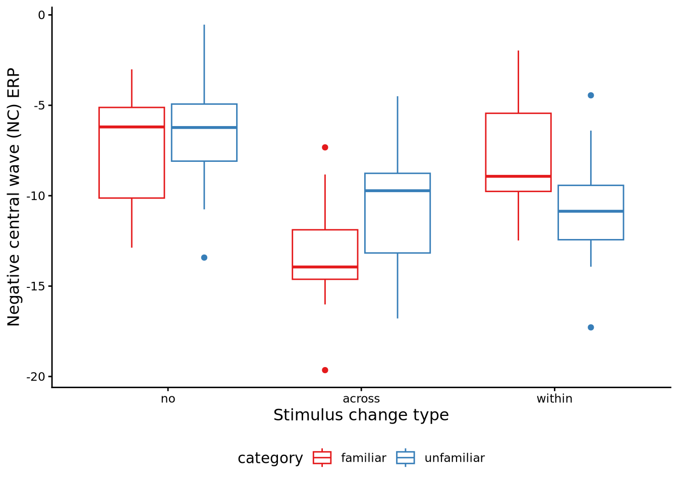
Here, we will analyse the data from an experiment described in Pomiechowska et al. (2021). This data set is available in sgsur as catknowledge, and is also shown in Table Table 10.2. In the experiment, \(J=24\) infants were shown objects that were momentarily occluded from their view. When they were occluded, the objects were either replaced with another object from the same category of object, or were replaced by an object from another category, or stayed the same. The infants were divided evenly into two conditions. In one condition, the infants were shown familiar categories of objects (e.g., balls, bottles, cars), and in the other condition, they were shown unfamiliar categories (e.g., feathers, guitars, hedgehogs). The purpose of the experiment was to test if children are better able to perceive changes across categories (i.e. when an object of one category is replaced with an object of a different category), or within categories (i.e. when an object of one category is replaced with an object from the same category). The main hypothesis being tested was that infants would be better able to perceive within-category changes if the category was unfamiliar than if it were familiar. Their measure of change detection was a brain activity event-related potential (ERP) known as the negative central wave (Nc). The data from this experiment is illustrated in Figure 10.5.
This ANOVA can be conducted in R with the aov_car command from the afex package as follows:
M_10_4 <- aov_car(nc_erp ~ category + Error(id/change), data = catknowledge)Note that the between-subjects variable, category (with values familiar and unfamiliar) is outside the Error function. Within the Error function, we have the subject indicator variable, id, and the within-subject variable change (with values no, across, and within). Although we do not explicitly indicate an interaction, using terms such as change:category or change*category, the interaction of change and category will be included in the model.
The output of this M_10_4 analysis will be almost identical in form to that of M_10_3, and so we may review it more briefly here to avoid repetition with our description of the output of M_10_3. First, let us look at the summary output first:
summary(M_10_4)
Univariate Type III Repeated-Measures ANOVA Assuming Sphericity

                Sum Sq num Df Error SS den Df  F value    Pr(>F)
(Intercept)     6303.5      1   424.67     22 326.5472 1.098e-14 ***
category           1.9      1   424.67     22   0.0971   0.75828
change           302.2      2   308.04     44  21.5828 2.940e-07 ***
category:change   98.3      2   308.04     44   7.0196   0.00226 **
---
Signif. codes:  0 '***' 0.001 '**' 0.01 '*' 0.05 '.' 0.1 ' ' 1


Mauchly Tests for Sphericity

                Test statistic p-value
change                 0.96956 0.72279
category:change        0.96956 0.72279


Greenhouse-Geisser and Huynh-Feldt Corrections
 for Departure from Sphericity

                 GG eps Pr(>F[GG])
change          0.97045  4.193e-07 ***
category:change 0.97045   0.002521 **
---
Signif. codes:  0 '***' 0.001 '**' 0.01 '*' 0.05 '.' 0.1 ' ' 1

                  HF eps   Pr(>F[HF])
change          1.062883 2.940122e-07
category:change 1.062883 2.259852e-03
At the top is the ANOVA table providing the \(F\) test results for each of the three hypotheses. As with M_10_3, the null hypothesis test that \(\theta = 0\) is also provided (first row of ANOVA table), but this is unlikely to ever be of real interest. Following this, we are provided with the results of the Mauchly test for sphericity, the Greenhouse-Geisser \(\hat{\epsilon}\) corrections, and the Huynh-Feldt \(\tilde{\epsilon}\) corrections. Note that no such result is provided for the change variable. This is not because it has only two levels, but because it is a between-subjects factor. As was the case with M_10_3, ultimately we always just use the Greenhouse-Geisser \(\hat{\epsilon}\) to adjust the degrees of freedom in the \(F\) tests.
Although the details in the summary output are important, all the vital information is provided by the nice summary, which can be obtained either by nice(M_10_4) or simply by typing M_10_4:
M_10_4Anova Table (Type 3 tests)
Response: nc_erp
Effect df MSE F ges p.value
1 category 1, 22 19.30 0.10 .003 .758
2 change 1.94, 42.70 7.21 21.58 *** .292 <.001
3 category:change 1.94, 42.70 7.21 7.02 ** .118 .003
---
Signif. codes: 0 '***' 0.001 '**' 0.01 '*' 0.05 '+' 0.1 ' ' 1
Sphericity correction method: GG As we can see, the interaction effect null hypothesis \(F\) test result is \(F(1.94, 42.7) = 7.02\), \(p = 0.003\), \(\hat{\epsilon}= 0.97\), \(\eta_{G}^2= 0.118\). The result for the null hypothesis test for the main effect of category is \(F(1, 22) = 0.1\), \(p = 0.758\), \(\eta_{G}^2= 0.003\), and the result for the test of the main effect of the change variable is \(F(1.94, 42.7) = 21.58\), \(p < 0.001\), \(\hat{\epsilon}= 0.97\), \(\eta_{G}^2= 0.292\).
Let us now examine the main effects. First, let us view the expected marginal means for each level of the change variable:
emmeans(M_10_4, ~ change) change emmean SE df lower.CL upper.CL
no -6.90 0.685 22 -8.32 -5.48
across -11.92 0.669 22 -13.30 -10.53
within -9.25 0.687 22 -10.68 -7.83
Results are averaged over the levels of: category
Confidence level used: 0.95 From this, the expected marginal means for three change types appear to be quite different. This is confirmed by looking at the pairwise differences with pairs():
pairs(emmeans(M_10_4, ~ change)) contrast estimate SE df t.ratio p.value
no - across 5.01 0.824 22 6.086 <0.0001
no - within 2.35 0.711 22 3.305 0.0087
across - within -2.67 0.752 22 -3.543 0.0050
Results are averaged over the levels of: category
P value adjustment: tukey method for comparing a family of 3 estimates The main effect of the change variable, or the marginal means of this variable, cannot directly inform us about how the effect of the change variable differs with the category variable. To begin to address this, we can first perform a simple main effects analysis of the effect of the change variable for each different level of the category variable:
simple_main_effects(nc_erp ~ Error(id/change), by = category, data = catknowledge)# A tibble: 2 × 8
by IV `num Df` `den Df` MSE F ges `Pr(>F)`
<chr> <chr> <dbl> <dbl> <dbl> <dbl> <dbl> <dbl>
1 familiar change 1.65 18.1 7.91 20.1 0.428 0.0000509
2 unfamiliar change 1.74 19.2 8.59 9.23 0.266 0.00216 From this result, we see that the means of the change type are different in both the familiar and unfamiliar category conditions. We can follow up these results by examining the expected marginal means for the different change types separately for each level of the category variable.
emmeans(M_10_4, ~ change | category)category = familiar:
change emmean SE df lower.CL upper.CL
no -7.38 0.968 22 -9.39 -5.37
across -13.33 0.946 22 -15.29 -11.36
within -7.85 0.971 22 -9.86 -5.84
category = unfamiliar:
change emmean SE df lower.CL upper.CL
no -6.43 0.968 22 -8.43 -4.42
across -10.51 0.946 22 -12.47 -8.55
within -10.65 0.971 22 -12.67 -8.64
Confidence level used: 0.95 From these results, we see the means for the across and the within change types appear to be quite different in the familiar versus the unfamiliar category condition. This is more apparent if we look at the pairwise differences between the change types in both category conditions:
pairs(emmeans(M_10_4, ~ change | category))category = familiar:
contrast estimate SE df t.ratio p.value
no - across 5.947 1.17 22 5.104 0.0001
no - within 0.472 1.01 22 0.470 0.8862
across - within -5.475 1.06 22 -5.145 0.0001
category = unfamiliar:
contrast estimate SE df t.ratio p.value
no - across 4.083 1.17 22 3.504 0.0055
no - within 4.227 1.01 22 4.205 0.0010
across - within 0.144 1.06 22 0.135 0.9900
P value adjustment: tukey method for comparing a family of 3 estimates From this, we can see that, for example, the mean for across is \(5.475\) less than the mean for within when the category is familiar, which is a significant effect. By contrast, the mean for across is \(0.144\) greater than the mean for within when the category is unfamiliar, and this difference is not significant. This is one of the key results as it shows how changes across category are more perceptible than changes within category, but only if the category is familiar.
We can also view this from another perspective. First, we can perform a simple main effects analysis of the effect of the category condition for each level of the change variable:
simple_main_effects(nc_erp ~ category + Error(id), by = change, data = catknowledge)# A tibble: 3 × 8
by IV `num Df` `den Df` MSE F ges `Pr(>F)`
<chr> <chr> <dbl> <dbl> <dbl> <dbl> <dbl> <dbl>
1 no category 1 22 11.3 0.484 0.0215 0.494
2 within category 1 22 11.3 4.16 0.159 0.0535
3 across category 1 22 10.7 4.43 0.168 0.0469This shows that the familiar and unfamiliar categories have different average effects when the change is within or across categories. We may follow this up by looking at the means for each category condition separately for each type of change:
emmeans(M_10_4, ~ category | change)change = no:
category emmean SE df lower.CL upper.CL
familiar -7.38 0.968 22 -9.39 -5.37
unfamiliar -6.43 0.968 22 -8.43 -4.42
change = across:
category emmean SE df lower.CL upper.CL
familiar -13.33 0.946 22 -15.29 -11.36
unfamiliar -10.51 0.946 22 -12.47 -8.55
change = within:
category emmean SE df lower.CL upper.CL
familiar -7.85 0.971 22 -9.86 -5.84
unfamiliar -10.65 0.971 22 -12.67 -8.64
Confidence level used: 0.95 Note how the difference between the values for the familiar and unfamiliar category conditions are different when the change is across versus within category. This is more apparent in the pairwise analysis:
pairs(emmeans(M_10_4, ~ category | change))change = no:
contrast estimate SE df t.ratio p.value
familiar - unfamiliar -0.953 1.37 22 -0.696 0.4938
change = across:
contrast estimate SE df t.ratio p.value
familiar - unfamiliar -2.817 1.34 22 -2.105 0.0469
change = within:
contrast estimate SE df t.ratio p.value
familiar - unfamiliar 2.802 1.37 22 2.041 0.0535Here, we see that when the change is across condition the effect for the familiar category is \(2.817\) less than the effect for the unfamiliar category. By contrast, when the change is within condition the effect for the familiar category is \(2.802\) greater than the effect for the unfamiliar category.
10.4 Further reading
Geoff Cumming’s Understanding The New Statistics (Cumming, 2013) devotes substantial attention to repeated-measures designs, explaining sphericity, effect sizes, and confidence intervals for within-subject comparisons.
Keselman, Algina, and Kowalchuk’s “The analysis of repeated measures designs: A review” (Keselman et al., 2001) published in the British Journal of Mathematical and Statistical Psychology provides a comprehensive technical review of repeated-measures analysis approaches and their assumptions.
10.5 Chapter summary
- Repeated measures designs collect multiple observations from the same individuals under different conditions, violating the independence assumption of standard ANOVA because observations within individuals are correlated.
- One-way repeated measures ANOVA extends standard ANOVA by including a subject-specific random effect term that accounts for systematic between-person differences and within-person correlations.
- The model adds a subject term \(\phi_{s_i}\) to the standard ANOVA equation, capturing baseline differences between individuals that persist across all measurement occasions.
- Sphericity assumes that the variances of all pairwise differences between conditions are equal, with violations inflating Type I error rates by making F-tests overly liberal.
- Mauchly’s test assesses sphericity but has low power in small samples, making routine application of Greenhouse-Geisser or Huynh-Feldt corrections advisable to adjust degrees of freedom when sphericity may be violated.
- Two-way repeated measures ANOVA handles designs with two within-subject factors, including their main effects and interaction, requiring additional random effect terms for subject-by-factor interactions.
- Mixed designs combine within-subject factors (repeated measures) with between-subject factors (independent groups), allowing simultaneous examination of how effects vary both within and between individuals.
- Factorial repeated measures models include interactions testing whether the effect of one factor depends on the level of another factor, requiring conditional interpretation when interactions are statistically significant.
- Repeated measures ANOVA provides a structured framework for analysing correlated observations while controlling family-wise error rates across pairwise comparisons, though it requires balanced data and sphericity assumptions that more flexible multilevel models can relax.